Modelling the data

47.    The JECFA and JMPR (2020) stated that it is important that any software employed for BMD estimation be thoroughly tested, and the source code should be made publicly available to allow for reproducibility and transparency. They consider the software packages PROAST and the US EPA’s Benchmark Dose Software, BMDS sufficient to meet these criteria. EFSA also host a web-based application of PROAST (FAO/WHO, 2020).

48.    These software employ mathematical models to fit dose-response data along with a quantification of how well the model has performed in fitting a user’s data to provide an estimation of the BMD along with a measure of the uncertainty. JECFA/JMPR noted there is no preference or hierarchy for the use of any one of these software over another, but transparency and clarity in the use and methods when using the software is important (FAO/WHO, 2020). 

Choosing an appropriate benchmark response

49.    The predefined selection of a degree of change that defines a level of response that is measurable, adverse and relevant to humans or the model species is known as the benchmark response or BMR (FAO/WHO, 2020). The related term, critical effect size (CES) is also employed in this context to refer to a clearly adverse BMR. Specifically, a CES is the maximum (change in the) magnitude of a specific (combination of) toxicological effect parameter(s) which is assumed to be non-adverse (Dekkers et al., 2001).

50.    Toxicological considerations such as the “meaningfulness” of a biological response or what biological response may be considered “adverse” may influence the choice of BMR level chosen. For instance, a 5% change would likely be less serious for a serum enzyme, which may increase at most 2-3 fold at some high exposure level, than it would be for a measurement of relative liver weight change (EFSA Workshop, 2023). Similarly, statistical considerations, such as when considering studies with relatively large within-group variation might lead a user to choose a BMR higher than 5% for endpoints (EFSA, 2017). 

51.    For continuous data, where there is no consensus as to the degree of change that is adverse, EFSA recommend a BMR of 5% to be set as a default which could be modified based on toxicological or statistical considerations (EFSA, 2017). In support of this choice of BMR, EFSA noted that analysis of a large number of studies from the US National Toxicology Program (US NTP) involving continuous data show that the BMDL for a BMR of 5% was, on average, close to the NOAEL derived from the same data set (for most individual data sets, the BMDL05 and NOAEL differed by an order of magnitude or less (Bokkers and Slob, 2007). EFSA also noted that similar observations were made in studies of fetal weight data (Kavlock et al., 1995).

52.    In contrast, the EPA recommend the BMR be set in terms of a change relative to the standard deviation of the data, rather than setting a percent of the biological response. They argued that this provides a standardised basis for analysis. However, they suggested that the ideal means of setting the BMR is having a biological basis for this decision, or some agreed definition of what minimal level of change is biologically significant (US EPA, 2012).

53.    For quantal data, the current recommendation from EFSA and US EPA is to employ a BMR of 10% when modelling. The selection of this response level is both statistical and practical based (EFSA, 2017; US EPA, 2012). The EPA note that this is near the limit of sensitivity for most cancer and noncancer bioassays of comparable size. However, in some cases biological considerations may warrant the use of a lower BMR (e.g., frank effects) (US EPA, 2012). EFSA also note that estimates from NOAEL studies, indicate the upper bounds of extra risk at the NOAEL are close to 10%, suggesting a BMR of 10% would be an appropriate default (EFSA, 2017) 

Choosing the correct model or models for the data

54.    Both the US EPA and EFSA emphasise using models, where possible, that are consistent with the biological processes understood to underlie the data. These biologically based descriptions of the data would ideally describe the essential toxicokinetic and toxicodynamic processes related to the specific compound and toxicological process (EFSA, 2022; US EPA, 2012). 

55.    In practice however, the biological mechanisms are often unknown. Finding the “best” mathematical model that describes the data is therefore a curve-fitting exercise that models the behaviour of experimentally measured endpoints in lieu of describing the underlying biology. Significant discussion exists around how to choose the most appropriate mathematical model(s) for this process (EFSA, 2022; FAO/WHO, 2020; US EPA, 2012). 

56.    In the absence of a biologically based model, the current guidance from the US EPA, JECFA and EFSA, is that no a priori preferences for any model types over another is recommended, unless there are justifiable reasons. When considering which model to apply to a given set of outcome data, the choice of model or group of models therefore is primarily determined by the nature of data making up the endpoint of interest and the experimental design, dose selection etc. used to generate the data (EFSA, 2022; FAO/WHO, 2020; US EPA, 2012). 

57.    This does not preclude a preference being made in practice. The US EPA guidance notes that as more flexible models are developed that can handle a variety of data types and qualities, hierarchies for some categories of endpoints will likely become more feasible and common. They noted as an example, the practice of US EPA’s IRIS program which preferentially employs a multistage model for cancer dose-response modelling of cancer bioassay data (Gehlhaus et al., 2011). This model is considered to be sufficiently flexible to be used across most cancer bioassay data and allows for greater consistency across cancer dose-response analyses (US EPA, 2012).

Models for continuous data

58.    DRMs for continuous data describe how the magnitude of response changes with dose and is typically defined as the central tendency of the observed data in relation to dose. Typical endpoints associated with continuous data include body weight and haematological parameters. Continuous data can be modelled using either individual values or summary statistics, if they describe the mean and variability at each dose level and the number of subjects per dose group (FAO/WHO, 2020).

59.    In their 2009 opinion, EFSA recommended that continuous data be modelled using the exponential or Hill family of dose-response models. At that time, 5 exponential models were included: differing primarily in the number of variable parameters available. 4 models were used to represent the Hill family (EFSA, 2009). Supporting this, Slob & Setzer found that most continuous dose-response data is well described by either exponential or Hill models (Slob and Setzer, 2014). Similarly, the JECFA/JMPR guidance recommended that only models contained within the general family of the exponential and Hill models be used as the default, and that the use of models outside of these need to be well justified (FAO/WHO, 2020).

60.    In their 2017 guidance, EFSA reiterated their recommendation that continuous data be modelled using the exponential and the Hill models but advised using only those model versions with 3 and 4 parameters. The four parameters (a, b, c and d) are described below. They noted that, in their experience, models with fewer than 3 parameters tended to have BMD confidence intervals with low coverage when parameter d in the model is in reality unequal to one (EFSA, 2017). EFSA’s recommended models for continuous data contain up to four parameters in which:

a)    Is the response at dose 0, i.e., the base or background parameter.

b)    Is a parameter which reflects the potency of the chemical (or the sensitivity of the population), left shifter parameters indicate higher potency/higher sensitivity.

c)    Is the maximum change in response, compared to background response.

d)    Is a parameter reflecting the steepness of the curve (on log-dose scale).

The four parameters are summarised in Figure 4.

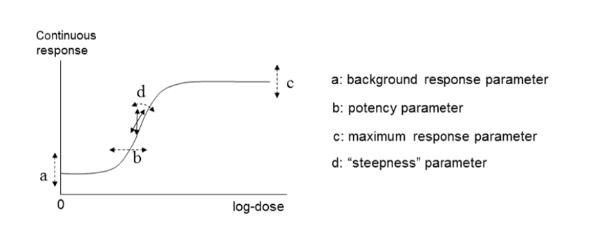
Four-model parameter: a, b, c and d and their interpretation for continuous data. This figure is black and white, and is made up of 2 sections. A graph on the left and a a list of each parameter.

Figure 4. A four-model parameter: a, b, c and d and their interpretation for continuous data. The dashed arrow indicates how the curve would change when changing the respective parameters (Figure taken from EFSA, 2017).

61.    The US EPA software, BMDS, includes exponential and Hill models for the analysis of continuous data. They also include additional models: the power and polynomial (including linear) model (US EPA, 2022). There is some disagreement on the use of these latter models, however. In their 2017 guidance, EFSA recommended against using these models on the grounds that they are additive with respect to the background response. This could lead to fitted curves which predict negative values (EFSA, 2017). 

62.    In EFSA’s most recent guidance (2022), the list of candidate models has been significantly updated and expanded. Along with exponential and Hill models, alternative flexible models (Inverse exponential, Log-normal, Gamma, LMS Two-stage, Probit, and Logistic) were added. This also unified the selection of models across both type of data, continuous and quantal. The current set includes 8 candidate models with 2 distributions for each (normal and Log normal) for a total of 16 models (default within the PROAST software) that can be fitted to the same data. All 16 models have 5 parameters (4 parameters for the mean, μ(x), and one for the variance parameter, σ2). This approach is significantly more liberal in the types and number of mathematical models allowed (EFSA, 2022). EFSA’s justification for this expansion is that the suite of models should contain a sufficiently large number of (diverse) models which are flexible enough to ensure at least one approximates the true unknown DRM well. With the current suite, they argue, the likelihood of finding at least one well-fitting model is high (EFSA, 2022). A full description of these models is provided in Annex B.

Models for dichotomous (quantal) data

63.    Dichotomous data, also referred to as quantal or binary data, describe an effect that is either observed or not observed in each individual subject such as a laboratory animal or human. Histopathology data, for instance, are a common type of dichotomous data (FAO/WHO, 2020). DRMs for quantal data define the probability that there will be an adverse response at a given dose, according to the occurrence of a particular adverse event. (EFSA, 2022). Similar to continuous data, DRMs for dichotomous or quantal data estimate the central tendency of these frequencies, which can be interpreted as the probability that the outcome will be observed in a population (FAO/WHO, 2020).

64.    Although the US EPA does not recommend specific models, US EPA practice can be inferred based on the models in BMDS (Haber et al., 2018). The US EPA software, BMDS, includes nine dichotomous models: Gamma, Logistic, Log-Logistic, Log Probit, Multistage, Probit, Weibull, Quantal Linear and Dichotomous Hill models (US EPA, 2022, 2012). By contrast, EFSA, in their 2017 guidance, list a total of eight candidate models for dichotomous endpoints. This list is largely a subgroup of the BMDS models, with two differences. Firstly, EFSA include latent variable models which are premised on an underlying continuous response, and dichotomised based on a cutoff value that is estimated from the data. In addition, EFSA recommends only the two-stage version of the linearised multistage (LMS) model, while BMDS allows for higher stages (multistage) (EFSA, 2017). 

65.    In their 2009 and 2017 guidance, EFSA set out separate sets of models for continuous and dichotomous endpoints, taking account of the distinct nature of the endpoints (EFSA, 2017, 2009). As discussed above, the most recent guidance (2022) updates these recommendations to a single set of candidate models for quantal and continuous data. The main difference between applying these models to quantal data is that there is only one possible distribution for a quantal endpoint: the Bernoulli distribution. This is a discrete distribution having two possible outcomes: n=0 and n=1, where n=1 ("occurs") occurs with probability p and n=0 ("does not occur") occurs with probability q=1-p, where 0<p<1. In chemical toxicology, such a distribution might describe the probability of a discrete adverse outcome such as animal death or presence of tumours i.e. it occurs or does not occur (EFSA, 2022). A fuller description of these models is provided in Annex B.

Other types of models

66.    There are also two special models: the full (or saturated) model and the null model. 
•    The null model describes the situation that there is no dose-response trend; i.e. the trend is flat / a horizontal line (EFSA, 2017). 
•    The full model, in contrast, expresses the dose-response relationship of the observed responses at the given doses, but does not assume any one specific dose-response. It does, however, include the relevant distributional part of the model (EFSA, 2017).

67.    In practice, these are useful reference models. The goodness of a particular fit can be evaluated by comparison with either the null model, to determine if there exists a dose-response trend, and also the full model, to ascertain the general goodness of fit (FAO/WHO, 2020).

68.    Ordinal data is a categorical data type where the variables constitute qualitative data but with a ranked order. Examples in chemical risk assessment might be pathological descriptions of the severity of an endpoint (e.g. minimal, mild, moderate, etc.). Ordinal data can be sometimes reduced to quantal data but this may result in a loss of information, which is not recommended (EFSA, 2022; FAO/WHO, 2020). Models for analysing ordinal data are available in different software packages, such as PROAST or CatReg (available from the EPA website (US EPA, 2017). 

69.    Nested data are commonly encountered in developmental toxicity studies. Litter effects are often related to the physiology of the mother. Therefore, statistical models should account for this, and analyses should be conducted on a per litter rather than a per pup basis, as the individual responses (e.g. presence of an adverse effect in a fetus) are inextricably linked to the group/nested unit (i.e. the litter) and therefore not statistically independent (US EPA, 2012). Models for nested data are currently available in the US EPA’s BMDS software, but not in PROAST. In the most recent BMDS software (Ver 3.3), only one nested dichotomous model is available (older versions included additional models). The nested logistic model is a log-logistic model, modified to include a litter-specific covariate. There are currently no models for nested continuous endpoints in the current BMDS software however such models are planned for a future release (US EPA, 2022). In their 2018 review of BMD modelling, Haber et al., compared the results of BMD calculations obtained using EFSA standard dichotomous models with their own analysis using the US EPA BMDS models for nested data for the derivation of an oral toxicity reference value for nickel. Use of the models for nested data in this case provided a better estimate of the BMDL, by using more of the data, and was more health-protective even though the BMDL was higher than that calculated using the standard models (Haber et al., 2018).

70.    For types of outcome and incidence data where there is not a standard set of models, there is no agreed guidance on the procedure. JECFA states that, where applicable, models can be selected from the literature. They warn however, that many models may not have been applied in a risk context. When choosing such a model or models, the choice and rationale for choosing should be clearly described including the reasons for including or excluding specific models (FAO/WHO, 2020).