Benchmark dose modelling in a UK chemical risk assessment framework
On this page
Skip the menu of subheadings on this page.This is a paper for discussion.
This does not represent the views of the Committee and should not be cited.
Introduction
1. In 2021 (TOX/2021/1) as part of a horizon scanning exercise, the Committee on Toxicity of Chemicals in Food, Consumer Products and the Environment (COT) identified the UK in future may need benchmark dose (BMD) modelling guidance. It was stated that in order that there is consistency in the implementation and in the interpretation of the BMD outputs, it is essential that there is guidance from a UK perspective. A COT (or wider UK) guidance document should be put together which would detail, amongst other things, a description of BMD modelling, including when it should be used; the software available and its respective limitations; and interpretation of the outputs. It should also list relevant resources with links. Discussions with experts in-the-field would likely be necessary to ensure that the guidance is accurate, reliable and future-proof for the Food Standards agency (FSA), COT and other relevant government departments (OGD).
2. Whilst carrying out its normal functions the COT is likely to come across instances where it will be essential that there is a good understanding of BMD modelling. The secretariat, in addition may also need to know how to carry out the modelling.
3. In 2022 (TOX/2022/07), as part of a horizon scanning exercise, the possibility of a workshop on BMD modelling was considered but it was agreed that a discussion paper would be most appropriate in the first instance.
4. Furthermore, in 2022 Members from COT, the Committee on Carcinogenicity of Chemicals in Food, Consumer Products and the Environment (COC) and the Committee on Mutagenicity of Chemicals in Food, Consumer Products and the Environment (COM) reviewed and discussed the recently published draft updated EFSA guidance on the BMD Approach; the most notable change being a move to use a Bayesian rather than frequentist approach in the modelling. In the discussion it was noted that the BMD was considered by EFSA to be scientifically more advanced than the NOAEL/LOAEL approach.
5. The Food Standards Agency (FSA) and COT are considering the use and practice of BMD as part of its ongoing evaluation of New Approach Methodologies (NAMs) in chemical risk assessment, within a UK food safety context for the safety of UK consumers.
6. This discussion paper provides information on the theory and practice of the BMD approach. The paper draws on previous evaluations by regulatory bodies and authorities (e.g. EFSA and US EPA). Furthermore, it includes a discussion of the areas of consensus and divergence between organisations and expert groups. It also highlights the work of the FSA Computational Fellow and describes a case study, that has used BMD modelling to derive a HBGV, as a proof of concept.
Background
7. The benchmark dose (BMD) approach was introduced almost 40 years ago as a more quantitative and informative estimate of the reference point (RP) from dose-response experiments. It was proposed as an alternative to the traditionally used No Observed Adverse Effect Level (NOAEL) or Lowest Observed Adverse Effect Level (LOAEL) (Crump, 1984).
8. The first established “safe dose” based on a BMD approach was for methylmercury, loaded onto the U.S. Environmental Protection Agency’s (EPA) Integrated Risk Information System (IRIS) in 1995 (Haber et al., 2018). In 2005, EFSA first recommended the BMD approach for deriving RPs for substances that are both genotoxic and carcinogenic (EFSA, 2005). In 2005, the World Health Organisation’s (WHO) International Programme on Chemical Safety (IPCS) published their “Principles for modelling dose-response for the risk assessment of chemicals” (FAO/WHO, 2005) and in 2006, the Joint Expert Committee on Food Additives (JECFA) began applying this approach for the safety evaluation of certain genotoxic and carcinogenic contaminants in food (FAO/WHO, 2006). Both the EPA and EFSA now recommend using the BMD approach, where appropriate, as the preferred methods to identify a RP for both genotoxic and non-genotoxic compounds (EFSA, 2017; US EPA, 2012).
9. Guidance on the BMD approach, including the statistical basis of the approach as well as technical guidance on its use and implementation have been provided by multiple authorities or committees (EFSA, 2022, 2017, 2009; FAO/WHO, 2020; US EPA, 2012) as well as many other reviews and discussions on the topic (Crump, 1984; Gephart et al., 2001; Haber et al., 2018; Slob, 2002).
Benchmark Dose Modelling in Chemical Risk assessment
Identifying a Reference Point from Toxicity studies
10. Hazard characterisation is a key step in the risk assessment pathway. It attempts to establish the nature and severity of (an) adverse effect(s) associated with exposure to a chemical, with particular attention paid to the relationship between the dose and effect (COT, 2020). Toxicity studies, carried out to characterise these adverse effects, are typically designed to identify a dose that can be used as a starting point for human health risk assessment. This dose is often referred to as the RP or the Point of Departure (PoD) (COT, 2020; EFSA, 2009).
11. Traditionally, RPs have been determined using the (NOAEL) or (LOAEL). The NOAEL (historically also sometimes referred to as a No Observed Effect level, NOEL) is a means of establishing a RP by determining the highest dose of a substance at which no (statistically) significant adverse effects are observed (FAO/WHO, 1990). While some variation exists in the statistical approaches, determination of the NOAEL typically involves multiple pairwise comparisons of the data at different doses, to an appropriate control data set. This approach can be used for data types including continuous data (i.e. data measured on a continuum, e.g., organ weight or blood biomarker concentration) or Dichotomous Data, also known as Quantal Data (i.e. Data where an effect may be classified into one of two possible outcomes, e.g., dead or alive, with or without incidence of a specific symptom such as tumours). Where statistically significant effects are detected at all dose levels tested, the lowest dose used in the study (i.e. the LOAEL) may be selected as the RP. In this case additional uncertainty factors are often recommended if the RP is used to produce a corresponding HBGV, in recognition of the fact that a lower dose may still cause an adverse effect. Conversely, if no statistically significant effect is observed at any of the dose levels, the highest dose is typically selected as the NOAEL (EFSA, 2022).
12. An alternate to the NOAEL/LOAEL is the BMD approach (Crump, 1984). The BMD is a dose level, estimated from a fitted dose-response curve or curves, associated with a pre-specified change in response (the benchmark response, BMR) relative to the control group (background response). Instead of comparing individual groups (doses), the BMD approach considers all the available dose-response data to estimate the shape of the overall dose-response relationship for a particular endpoint (Figure 1). It is possible to derive confidence levels of the BMD response from the dose-response modelling with the BMD lower confidence level (BMDL) typically taken as the RP for establishing HBGVs (EFSA, 2022).
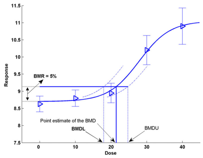
Illustration of the BMD approach using hypothetical continuous data. A chart depicted in black, blue and grey colours. Th bottom axis is: Dose and the side axis is: Response.
Figure 1. Illustration of the BMD approach using hypothetical continuous data (Figure taken from EFSA, 2017). Hypothetical experimental mean response data (triangles) are plotted along with their confidence intervals. The solid curve represents the fitted dose-response model. The curve determines the point estimate of the BMD, generally defined as a dose that corresponds to a low but measurable change in response, and here representing a benchmark response (BMR) of 5%. The dashed curves represent, respectively, the upper and lower 95% one-sided confidence bounds for the effect size as a function of dose. Their intersections with the horizontal line are at the lower and upper bounds of the BMD, denoted BMDL and BMDU, respectively.
13. Both the U.S. EPA and EFSA now recommend using the BMD approach, where appropriate, as the preferred means to identify a RP for deriving a HBGV. This is also the stated preference of the JECFA and JMPR (Joint FAO/WHO Meeting on Pesticide Residues).
Selected Previous Publications
14. The selected publications represent the existing guidance offered by both EFSA and the US EPA regarding implementation and recommended best practices for BMD modelling in chemical risk assessment, with specific reference to their respective BMD software, PROAST and BMDS. EFSA have published a number of opinions on BMD modelling since 2009 and although the US EPA have not published their own opinion document, their preferred practices can be inferred from their 2012 Technical Guidance Document for the application of their BMDS Benchmark Dose software.
EFSA 2005 - Opinion of the Scientific Committee on a request from EFSA related to A Harmonised Approach for Risk Assessment of Substances which are both Genotoxic and Carcinogenic
15. In 2005, EFSA’s Scientific Committee (SC) proposed a harmonised approach for risk assessments for substances that have both genotoxic and carcinogenic properties. EFSA expressed reservations about extrapolating from the typically high doses of genotoxic and carcinogenic substances to much lower levels to which humans are occasionally exposed.
16. EFSA noted that the selection of mathematical model was crucial and could lead to wide variation in the predicted threshold for safety. This often led to differing conclusions for the same substance, depending on the model chosen. They also noted that such approaches had little basis in rationality, as it was often unknown if the model chosen reflected the underlying biological processes.
17. EFSA recommended using a margin of exposure (MOE) approach using a reliable RP for the substance under consideration. They recommended the use of BMD modelling as a reliable means to obtain an RP. They concluded that BMD modelling was the superior approach as it used all the information obtained over the range of doses in the dataset chosen from which to establish the health-based guidance value. EFSA further recommended the use of the BMDL10 which would represent an estimate of the lowest dose which is 95% certain to cause no more than a 10% cancer incidence in rodents (EFSA, 2005).
EFSA 2009 - Guidance of the Scientific Committee on Use of the benchmark dose approach in risk assessment
18. In their 2009 guidance, EFSA considered the utility and practical application of BMD as a generalised tool for risk assessment. They concluded, that since BMD incorporates all the available dose-response data and provides a quantification of uncertainties in the dose-response, a BMD approach represents a scientifically more advanced method compared to the traditional NOAEL approach for deriving a RP. They also noted that while the BMD approach had occasionally been employed in risk assessments up to that point, no systematic approach to the use of the BMD existed.
19. EFSA reconfirmed both their view that an MOE approach was the most appropriate for risk assessment of substances that are both genotoxic and carcinogenic (EFSA, 2005) and the use of the BDML as the generally accepted RP. More generally, for chemical risk assessment, EFSA proposed that a default Benchmark response (BMR) value of 10% be used for quantal data and 5% for continuous data from animal studies, although this default BMR may be modified based on statistical or toxicological considerations.
20. EFSA rejected the suggestion that larger or additional uncertainty factors are needed if the BMDL is used as the RP. They concluded that HBGVs derived from the BMDL are expected to be as protective as those from the NOAEL approach, on average over many risk assessments. EFSA concluded that it was not necessary to repeat previous evaluations of safety using the new BMD approach. They concluded, based on similar reasoning, that the BMD and NOAEL would be, on average, as protective as one another over many risk assessments.
21. EFSA also recommended that any future updates to test guidelines, such as the OECD guidelines, should include a consideration of the BMD approach.
US EPA 2012 - Benchmark Dose (BMDS) Technical Guidance Document
22. In their 2012 document, the US EPA technical panel presented step-by-step guidance for the understanding and application of existing BMD methods in risk assessment. This included guidance on evaluating studies and endpoint types suitable for modelling, selecting appropriate BMR levels, model fitting and BMD computation, judging the fit of the model, and calculating the BMDL. Finally, the document provided several demonstrations of BMD and BMDL derivations from scientific data.
23. The guidance discussed general approaches for selecting the BMR levels but stopped short of recommending any particular value for the BMR being modelled. Instead, it recommended a flexible approach based on thorough consideration of the statistical and biological characteristics of the dataset and the applications for which the resulting BMDs/BMDLs will be used. The guidance recommended that selections be made on a case-by-case basis, and justification should be provided for each BMR selection. For quantal data however it suggested an extra risk of 10% as the BMR for standard reporting (to serve as a basis for comparisons across chemicals and endpoints). This is because the 10% response is near the limit of sensitivity in most cancer bioassays and in some noncancer bioassays.
24. Similarly, the guidance recommended a case-by-case approach for choosing an appropriate model or models to use in computing the BMD. In the absence of information about the biological basis of the dose response relationship, the document provides guidance on model selection and model fitting, as well as information on determining goodness-of-fit, and comparing models to decide which to use for obtaining the BMD and BMDL. The guidance provided general recommendations, including that α = 0.1 be used to compute the critical value for goodness-of-fit and that a graphical display of the model fit be examined as well. For comparison of models and selection of the model to use for BMD computation, the use of Akaike’s Information Criterion (AIC) is recommended.
25. The document does not advocate the use of any one software package. A discussion of the preferred computational algorithms is intended however, to provide users a computational or statistical basis to make an informed choice in the selection of software. It is recommended that software with well-documented methodology be used, such as the EPA’s BMDS package, from which it also provides worked example for the purpose of practical demonstration.
26. Reporting recommendations from the BMD/BMDL calculations are also discussed. This guidance lists several reporting recommendations for the BMD and BMDL. Finally, the guidance provided a generalised workflow and decision tree that can be adapted and implemented for the purpose of chemical risk assessment (Figure 2). A flow chart is provided to help visualise how the BMD approach fits within a larger risk assessment framework. In addition, a section outlining a “decision tree” is intended to guide the user in choosing the most appropriate BMD approach for their particular data and risk assessment.
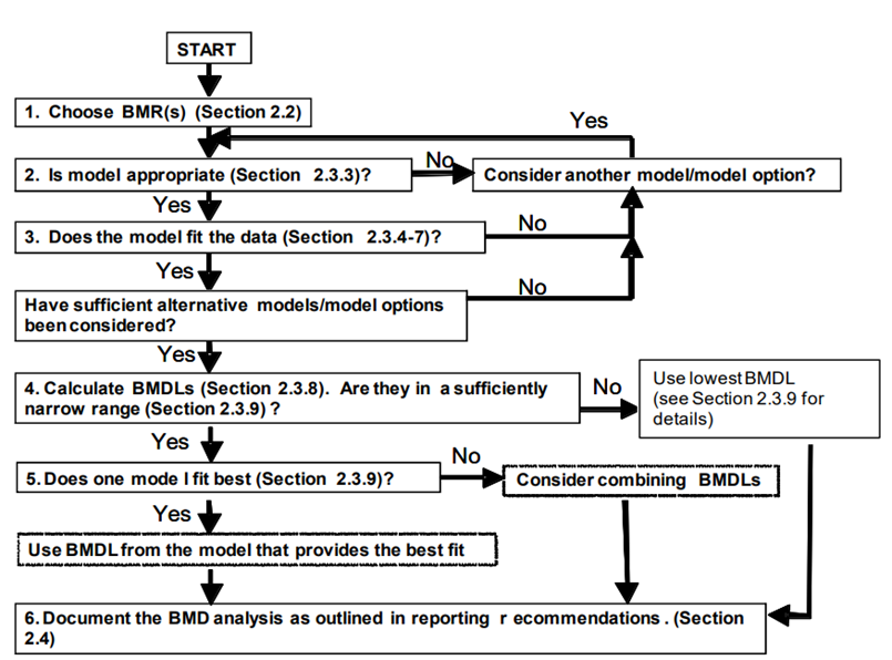
Decision tree summarising the generalised step-by-step approach to calculate the BMD and associated confidence intervals and BMDL. The tree is shown in black and white.
Figure 2. Decision tree summarising the generalised step-by-step approach to calculate the BMD and associated confidence intervals and BMDL (Image from US EPA, 2012).
EFSA 2017 - Update: use of the benchmark dose approach in risk assessment
27. EFSA’s 2017 document is an update of the 2009 guidance, informed by user experience with BMD application in regulatory risk assessment, and includes the latest methodological developments in BMD modelling. The update confirms many of the recommendations laid out in the 2009 guidance. EFSA reconfirmed their view that a BMD approach is a scientifically more advanced method compared to the NOAEL for identifying the RP and that HBGVs based on a BMD approach are expected to be as protective as those based on the NOAEL approach.
28. The most significant updates concern the application of the BMD approach in practice. Most notable are the developments in model averaging capabilities which EFSA now recommend as the preferred method for calculating the BMD confidence interval. A flowchart and worked examples have been inserted in this update to guide the reader step-by-step when performing a BMD analysis (Figure 3), as well as a chapter on the distributional part of dose-response models (DRM) and a template for reporting a BMD analysis in a complete and transparent manner.
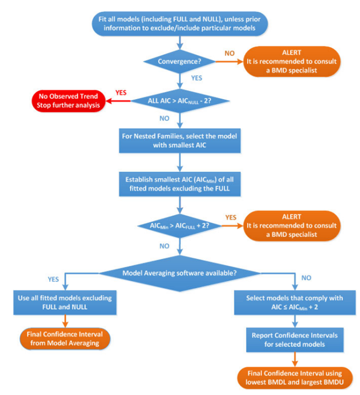
Flow chart to establish BMD confidence interval and BMDL for dose-response data set of a specified endpoint. The flow chart is in blue, red and orange. The text is written in white, blue, red and orange.
Figure 3. Flow chart to establish BMD confidence interval and BMDL for dose-response data set of a specified endpoint. AIC: Akaike information criterion; AICnull: AIC value of the Null Model; AICfull: AIC value of the Full Model; AICmin: AIC value of the model with the lowest AIC value, the null and full models being excluded (Image taken from EFSA, 2017).
29. The set of available default models has been reviewed and updated. For continuous data, both the exponential and Hill family of models are recommended (4 models total). For quantal data, 8 models are recommended: Logistic, Probit, Log-logistic, Log-probit, Weibull, Gamma, linearised multistage models (LMS) (two-stage) model and the Latent variable models (LVMs). To assess the relative goodness of fit of different mathematical models to the dose-response data set, the Akaike information criterion (AIC) is now the recommend approach.
30. EFSA propose that a BMD approach can be applied to all chemicals in food, independent of the nature or source. They conclude that the BMD modelling is also appropriate for dose-response data from epidemiological studies, although no explicit guidance is provided for this (EFSA, 2017).
EFSA 2022 - Guidance on the use of the benchmark dose approach in risk assessment
31. In 2022, EFSA published new guidance which considered the most recent developments in BMD modelling and aimed to better align EFSA’s approach with internationally agreed concepts and approaches.
32. EFSA reconfirmed its guidance and reasoning, set out in 2009 and 2017, regarding the recommendation of the BMD approach in chemical risk assessment. The set of default models for BMD analysis has been reviewed and updated, allowing a single set of models to be used for both quantal and continuous data. Model averaging is again recommended as the preferred method for evaluating the results from the choice of available models.
33. Of most significance is EFSAs recommendation to change from a frequentist to a Bayesian paradigm. Confidence and significance levels are replaced, in the Bayesian approach, by probability distributions attached to unknown modelling parameters. Credible intervals replace the frequentist use of confidence intervals. EFSA note that the Bayesian method allows the model to be updated with new or existing knowledge, allowing it to “mimic a learning process”. Finally, the step-by-step guidance and flowchart for BMD analysis has been updated in light of these changes, and a chapter comparing the frequentist and Bayesian paradigms has been inserted (EFSA, 2022).
COT previous discussions
JECFA/JMPR update of Chapter 5, EHC 240 (2020)
34. The COT were provided a summary of chapter 5 (dose-response assessment and derivation of health-based guidance values) of the “principles and methods for the risk assessment of chemicals in food, Environmental Health Criteria 240” (EHC 240) guidance document that was released by the World Health Organisation for public consultation (TOX/2020/01). Members of the Committee were invited to comment on the draft update.
35. Potential discrepancies between the descriptions of the benchmark dose approach and that by the Environmental Protection Agency were addressed.
36. Comparisons were made between the flow chart presented in Figure 1 of TOX/2020/01 and that used by EFSA (Figure 8 in 2017 Guidance); it was noted that the figures serve slightly different purposes and that the flow chart used by EFSA provides more detailed information on the conduct of dose-response modelling.
37. The Committee concluded that the methodologies of the updated draft chapter and the previous version were very similar, and the main differences were in the structure and detail of the chapter.
Updated EFSA guidance on the Benchmark Dose Approach (2022)
38. In March 2022, The Committee was informed of a meeting held between interested COT, COC and COM Members to discuss the recently published draft updated EFSA guidance on the Benchmark Dose Approach; the most notable change being a move to use a Bayesian rather than frequentist approach in the modelling.
39. In the discussion it was highlighted that the guidance on modelling took more account of statistical issues, rather than the underlying biology. It was noted that the benchmark dose was considered by EFSA to be scientifically more advanced than the NOAEL/LOAEL approach.
NOAEL approach vs BMD approach
40. Both EFSA and the US EPA consider the BMD approach to be the more quantitative and scientifically advanced approach to deriving the RP compared to the NOAEL approach. In theory, the BMD approach uses all the available dose-response information within a given dataset. The NOAEL approach, in contrast, effectively uses only the data that make up the control group and one other dose group: the NOAEL/LOAEL group (EFSA, 2017; US EPA, 2012).
41. An important acknowledgment is that the NOAEL approach is ostensibly designed to identify a “no effect” level for a given substance. Slob and others have argued that the NOAEL should more accurately be understood as the dose at which no statistically significant effect is detected. As Slob notes in a 2014 publication: “a prominent misconception about the NOAEL approach is that the NOAEL reflects a dose without effects”. In reality, the “true” NOAEL could be lower than the statistically determined NOAEL. Slob notes that the NOAEL is not substantively different from a BMD in this regard: they both reflect a dose where the true effect is small. The primary difference is that, in case of a NOAEL, the effect size is not defined (but assumed to be small), while for a BMDL, the effect is predefined, so it is known that the size of the effect at the BMDL is not larger than this specified value (i.e. the Benchmark response, BMR) (Slob, 2014).
42. As the BMD approach does not calculate a “no effect dose” but rather is set at a predefined effect size, it has been suggested that additional uncertainty factors might be appropriate when using a BMDL as the RP. In their 2017 guidance, EFSA argue that this concern is based on the false assumption that a NOAEL is associated with the complete absence of adverse effect. Furthermore, based on the data from National Toxicology Program (US NTP) studies (Bokkers and Slob, 2007), EFSA concluded that the default values of the BMR are such that the BMDL, on average, coincides with the NOAEL. They concluded that additional uncertainty factors, beyond those normally applied are not necessary and HBGVs derived using a BMDL as the RP can be expected, on average, to be as protective as those derived from the NOAELs (EFSA, 2017).
43. The reliability of the NOAEL approach is also crucially dependent on the sensitivity of the test method. The likelihood of detecting a small effect is directly proportional to the sample size being studied. The larger the sample size at a given dose, the more power in statistical terms there is to detect such an effect. This also results in the effect that studies performed with fewer animals per group will tend to yield a higher NOAEL than equivalent studies performed with higher numbers, due to decreased statistical sensitivity (EFSA, 2017). As noted by Haber et al., (2018) this is particularly undesirable in a regulatory context because it disincentivises better designed, larger studies in favour of smaller, less powerful ones.
44. The BMD approach also provides important information regarding the uncertainties in the data. The output of the BMD approach provides a quantitative assessment of data quality, as described by the confidence (or credible) intervals. In the NOAEL approach, experimental uncertainties resulting from, e.g. low study power or high variance, in the response effect are not captured (EFSA, 2022).
45. Another limitation of the NOAEL approach is the study design. As noted by Crump (1984), the NOAEL must necessarily be one of the study’s experimental doses. This artificially constrains NOAEL assignment to arbitrary doses which often are a poor reflection of the data. The advantage of the BMD approach, is that the BMD can be any dose level, including a dose between the assigned study doses (Crump, 1984). This is partly a result of traditional study design protocols in toxicology. At a recent EFSA workshop, it was noted that the current OECD guidance on designing animal experiments take, by default, the goal to be detecting statistical effect levels. Therefore animal studies often limit the number of doses to maximise the statistical power at each dose group (EFSA Workshop, 2023). Slob notes that the BMD approach therefore, theoretically allows for more efficient use of animals. More information is obtained from the same number of animals, or conversely, similar information may be obtained from fewer animals, compared with the NOAEL approach (Slob, 2014).
46. As the dose-response output for the BMD models is linked to a predefined biological effect size (rather than threshold of statistical significance) comparisons across potencies of different substances, or of the same substances under different conditions, is possible. For this reason, EFSA note that the BMD approach is also suitable for the derivation of relative potency factors (RPFs) or toxic equivalency factors (TEF) for individual substances in a mixture that share a common mode of toxicological action (EFSA, 2017). For example, the BMD approach has been used to provide relative potency estimates for different organophosphates in toxicological studies (Bosgra et al., 2009).
Modelling the data
47. The JECFA and JMPR (2020) stated that it is important that any software employed for BMD estimation be thoroughly tested, and the source code should be made publicly available to allow for reproducibility and transparency. They consider the software packages PROAST and the US EPA’s Benchmark Dose Software, BMDS sufficient to meet these criteria. EFSA also host a web-based application of PROAST (FAO/WHO, 2020).
48. These software employ mathematical models to fit dose-response data along with a quantification of how well the model has performed in fitting a user’s data to provide an estimation of the BMD along with a measure of the uncertainty. JECFA/JMPR noted there is no preference or hierarchy for the use of any one of these software over another, but transparency and clarity in the use and methods when using the software is important (FAO/WHO, 2020).
Choosing an appropriate benchmark response
49. The predefined selection of a degree of change that defines a level of response that is measurable, adverse and relevant to humans or the model species is known as the benchmark response or BMR (FAO/WHO, 2020). The related term, critical effect size (CES) is also employed in this context to refer to a clearly adverse BMR. Specifically, a CES is the maximum (change in the) magnitude of a specific (combination of) toxicological effect parameter(s) which is assumed to be non-adverse (Dekkers et al., 2001).
50. Toxicological considerations such as the “meaningfulness” of a biological response or what biological response may be considered “adverse” may influence the choice of BMR level chosen. For instance, a 5% change would likely be less serious for a serum enzyme, which may increase at most 2-3 fold at some high exposure level, than it would be for a measurement of relative liver weight change (EFSA Workshop, 2023). Similarly, statistical considerations, such as when considering studies with relatively large within-group variation might lead a user to choose a BMR higher than 5% for endpoints (EFSA, 2017).
51. For continuous data, where there is no consensus as to the degree of change that is adverse, EFSA recommend a BMR of 5% to be set as a default which could be modified based on toxicological or statistical considerations (EFSA, 2017). In support of this choice of BMR, EFSA noted that analysis of a large number of studies from the US National Toxicology Program (US NTP) involving continuous data show that the BMDL for a BMR of 5% was, on average, close to the NOAEL derived from the same data set (for most individual data sets, the BMDL05 and NOAEL differed by an order of magnitude or less (Bokkers and Slob, 2007). EFSA also noted that similar observations were made in studies of fetal weight data (Kavlock et al., 1995).
52. In contrast, the EPA recommend the BMR be set in terms of a change relative to the standard deviation of the data, rather than setting a percent of the biological response. They argued that this provides a standardised basis for analysis. However, they suggested that the ideal means of setting the BMR is having a biological basis for this decision, or some agreed definition of what minimal level of change is biologically significant (US EPA, 2012).
53. For quantal data, the current recommendation from EFSA and US EPA is to employ a BMR of 10% when modelling. The selection of this response level is both statistical and practical based (EFSA, 2017; US EPA, 2012). The EPA note that this is near the limit of sensitivity for most cancer and noncancer bioassays of comparable size. However, in some cases biological considerations may warrant the use of a lower BMR (e.g., frank effects) (US EPA, 2012). EFSA also note that estimates from NOAEL studies, indicate the upper bounds of extra risk at the NOAEL are close to 10%, suggesting a BMR of 10% would be an appropriate default (EFSA, 2017)
Choosing the correct model or models for the data
54. Both the US EPA and EFSA emphasise using models, where possible, that are consistent with the biological processes understood to underlie the data. These biologically based descriptions of the data would ideally describe the essential toxicokinetic and toxicodynamic processes related to the specific compound and toxicological process (EFSA, 2022; US EPA, 2012).
55. In practice however, the biological mechanisms are often unknown. Finding the “best” mathematical model that describes the data is therefore a curve-fitting exercise that models the behaviour of experimentally measured endpoints in lieu of describing the underlying biology. Significant discussion exists around how to choose the most appropriate mathematical model(s) for this process (EFSA, 2022; FAO/WHO, 2020; US EPA, 2012).
56. In the absence of a biologically based model, the current guidance from the US EPA, JECFA and EFSA, is that no a priori preferences for any model types over another is recommended, unless there are justifiable reasons. When considering which model to apply to a given set of outcome data, the choice of model or group of models therefore is primarily determined by the nature of data making up the endpoint of interest and the experimental design, dose selection etc. used to generate the data (EFSA, 2022; FAO/WHO, 2020; US EPA, 2012).
57. This does not preclude a preference being made in practice. The US EPA guidance notes that as more flexible models are developed that can handle a variety of data types and qualities, hierarchies for some categories of endpoints will likely become more feasible and common. They noted as an example, the practice of US EPA’s IRIS program which preferentially employs a multistage model for cancer dose-response modelling of cancer bioassay data (Gehlhaus et al., 2011). This model is considered to be sufficiently flexible to be used across most cancer bioassay data and allows for greater consistency across cancer dose-response analyses (US EPA, 2012).
Models for continuous data
58. DRMs for continuous data describe how the magnitude of response changes with dose and is typically defined as the central tendency of the observed data in relation to dose. Typical endpoints associated with continuous data include body weight and haematological parameters. Continuous data can be modelled using either individual values or summary statistics, if they describe the mean and variability at each dose level and the number of subjects per dose group (FAO/WHO, 2020).
59. In their 2009 opinion, EFSA recommended that continuous data be modelled using the exponential or Hill family of dose-response models. At that time, 5 exponential models were included: differing primarily in the number of variable parameters available. 4 models were used to represent the Hill family (EFSA, 2009). Supporting this, Slob & Setzer found that most continuous dose-response data is well described by either exponential or Hill models (Slob and Setzer, 2014). Similarly, the JECFA/JMPR guidance recommended that only models contained within the general family of the exponential and Hill models be used as the default, and that the use of models outside of these need to be well justified (FAO/WHO, 2020).
60. In their 2017 guidance, EFSA reiterated their recommendation that continuous data be modelled using the exponential and the Hill models but advised using only those model versions with 3 and 4 parameters. The four parameters (a, b, c and d) are described below. They noted that, in their experience, models with fewer than 3 parameters tended to have BMD confidence intervals with low coverage when parameter d in the model is in reality unequal to one (EFSA, 2017). EFSA’s recommended models for continuous data contain up to four parameters in which:
a) Is the response at dose 0, i.e., the base or background parameter.
b) Is a parameter which reflects the potency of the chemical (or the sensitivity of the population), left shifter parameters indicate higher potency/higher sensitivity.
c) Is the maximum change in response, compared to background response.
d) Is a parameter reflecting the steepness of the curve (on log-dose scale).
The four parameters are summarised in Figure 4.
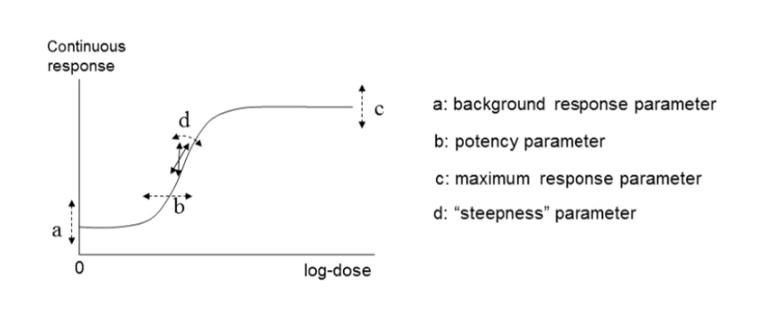
Four-model parameter: a, b, c and d and their interpretation for continuous data. This figure is black and white, and is made up of 2 sections. A graph on the left and a a list of each parameter.
Figure 4. A four-model parameter: a, b, c and d and their interpretation for continuous data. The dashed arrow indicates how the curve would change when changing the respective parameters (Figure taken from EFSA, 2017).
61. The US EPA software, BMDS, includes exponential and Hill models for the analysis of continuous data. They also include additional models: the power and polynomial (including linear) model (US EPA, 2022). There is some disagreement on the use of these latter models, however. In their 2017 guidance, EFSA recommended against using these models on the grounds that they are additive with respect to the background response. This could lead to fitted curves which predict negative values (EFSA, 2017).
62. In EFSA’s most recent guidance (2022), the list of candidate models has been significantly updated and expanded. Along with exponential and Hill models, alternative flexible models (Inverse exponential, Log-normal, Gamma, LMS Two-stage, Probit, and Logistic) were added. This also unified the selection of models across both type of data, continuous and quantal. The current set includes 8 candidate models with 2 distributions for each (normal and Log normal) for a total of 16 models (default within the PROAST software) that can be fitted to the same data. All 16 models have 5 parameters (4 parameters for the mean, μ(x), and one for the variance parameter, σ2). This approach is significantly more liberal in the types and number of mathematical models allowed (EFSA, 2022). EFSA’s justification for this expansion is that the suite of models should contain a sufficiently large number of (diverse) models which are flexible enough to ensure at least one approximates the true unknown DRM well. With the current suite, they argue, the likelihood of finding at least one well-fitting model is high (EFSA, 2022). A full description of these models is provided in Annex B.
Models for dichotomous (quantal) data
63. Dichotomous data, also referred to as quantal or binary data, describe an effect that is either observed or not observed in each individual subject such as a laboratory animal or human. Histopathology data, for instance, are a common type of dichotomous data (FAO/WHO, 2020). DRMs for quantal data define the probability that there will be an adverse response at a given dose, according to the occurrence of a particular adverse event. (EFSA, 2022). Similar to continuous data, DRMs for dichotomous or quantal data estimate the central tendency of these frequencies, which can be interpreted as the probability that the outcome will be observed in a population (FAO/WHO, 2020).
64. Although the US EPA does not recommend specific models, US EPA practice can be inferred based on the models in BMDS (Haber et al., 2018). The US EPA software, BMDS, includes nine dichotomous models: Gamma, Logistic, Log-Logistic, Log Probit, Multistage, Probit, Weibull, Quantal Linear and Dichotomous Hill models (US EPA, 2022, 2012). By contrast, EFSA, in their 2017 guidance, list a total of eight candidate models for dichotomous endpoints. This list is largely a subgroup of the BMDS models, with two differences. Firstly, EFSA include latent variable models which are premised on an underlying continuous response, and dichotomised based on a cutoff value that is estimated from the data. In addition, EFSA recommends only the two-stage version of the linearised multistage (LMS) model, while BMDS allows for higher stages (multistage) (EFSA, 2017).
65. In their 2009 and 2017 guidance, EFSA set out separate sets of models for continuous and dichotomous endpoints, taking account of the distinct nature of the endpoints (EFSA, 2017, 2009). As discussed above, the most recent guidance (2022) updates these recommendations to a single set of candidate models for quantal and continuous data. The main difference between applying these models to quantal data is that there is only one possible distribution for a quantal endpoint: the Bernoulli distribution. This is a discrete distribution having two possible outcomes: n=0 and n=1, where n=1 ("occurs") occurs with probability p and n=0 ("does not occur") occurs with probability q=1-p, where 0<p<1. In chemical toxicology, such a distribution might describe the probability of a discrete adverse outcome such as animal death or presence of tumours i.e. it occurs or does not occur (EFSA, 2022). A fuller description of these models is provided in Annex B.
Other types of models
66. There are also two special models: the full (or saturated) model and the null model.
• The null model describes the situation that there is no dose-response trend; i.e. the trend is flat / a horizontal line (EFSA, 2017).
• The full model, in contrast, expresses the dose-response relationship of the observed responses at the given doses, but does not assume any one specific dose-response. It does, however, include the relevant distributional part of the model (EFSA, 2017).
In practice, these are useful reference models. The goodness of a particular fit can be evaluated by comparison with either the null model, to determine if there exists a dose-response trend, and also the full model, to ascertain the general goodness of fit (FAO/WHO, 2020).
67. Ordinal data is a categorical data type where the variables constitute qualitative data but with a ranked order. Examples in chemical risk assessment might be pathological descriptions of the severity of an endpoint (e.g. minimal, mild, moderate, etc.). Ordinal data can be sometimes reduced to quantal data but this may result in a loss of information, which is not recommended (EFSA, 2022; FAO/WHO, 2020). Models for analysing ordinal data are available in different software packages, such as PROAST or CatReg (available from the EPA website (US EPA, 2017).
68. Nested data are commonly encountered in developmental toxicity studies. Litter effects are often related to the physiology of the mother. Therefore, statistical models should account for this, and analyses should be conducted on a per litter rather than a per pup basis, as the individual responses (e.g. presence of an adverse effect in a fetus) are inextricably linked to the group/nested unit (i.e. the litter) and therefore not statistically independent (US EPA, 2012). Models for nested data are currently available in the US EPA’s BMDS software, but not in PROAST. In the most recent BMDS software (Ver 3.3), only one nested dichotomous model is available (older versions included additional models). The nested logistic model is a log-logistic model, modified to include a litter-specific covariate. There are currently no models for nested continuous endpoints in the current BMDS software however such models are planned for a future release (US EPA, 2022). In their 2018 review of BMD modelling, Haber et al., compared the results of BMD calculations obtained using EFSA standard dichotomous models with their own analysis using the US EPA BMDS models for nested data for the derivation of an oral toxicity reference value for nickel. Use of the models for nested data in this case provided a better estimate of the BMDL, by using more of the data, and was more health-protective even though the BMDL was higher than that calculated using the standard models (Haber et al., 2018).
69. For types of outcome and incidence data where there is not a standard set of models, there is no agreed guidance on the procedure. JECFA states that, where applicable, models can be selected from the literature. They warn however, that many models may not have been applied in a risk context. When choosing such a model or models, the choice and rationale for choosing should be clearly described including the reasons for including or excluding specific models (FAO/WHO, 2020).
Fitting the model to the data
70. The objective of model fitting is to best describe the dose-response relationship of a given data set. The process typically involves searching for parameter values in the model that lead to a function or curve that describes the data well, using some statistical criterion that defines a good fit (FAO/WHO, 2020).
Constraining or not constraining the models
71. As curve fitting typically optimise a model’s “best fit” to a given set of data without knowledge of the biological dose-response, this may lead to model fits that describe the data well but contain parameter values which are “biologically improbable”. It has been argued that setting parameter bounds adds information which may improve the accuracy of the model and mitigate the likelihood of biologically implausible responses (FAO/WHO, 2020).
72. Some constraints serve a practical necessity e.g., constraining the probabilities of an effect in a dichotomous model to no greater than one (US EPA, 2012). The EPA and EFSA agree on other general restrictions such as biological measures generally being positive, and that dose-responses will be generally monotonic (i.e., a higher dose of a given substance will have an equal or greater effect than a lower dose). Much existing practice constrains models to avoid non-monotonic curves (EFSA, 2017; US EPA, 2012).
73. Other model restraints are controversial, and guidance from the EPA and EFSA diverge (Haber et al., 2018). An example is constraining models that are steeply supralinear. In some models, such as the Weibull model, where the dose is raised to a power of a given parameter, the slope of the dose-response curve can become very steep at low doses if the power parameter is estimated at values lower than 1. Thus, the US EPA recommends that the modeler should consider constraining power parameters to be 1 or greater (this is the default in the BMDS software). While EFSA (2017) acknowledge this concern exists, they point to work by Slob and Setzer (2014) that demonstrates that this constraint is largely based on a false argument and is contradicted by real dose-response data (EFSA, 2017; Slob and Setzer, 2014). They recommend against constraining the model in this way, as it could produce artificially high BMDLs (EFSA, 2017).
74. The US EPA encourages the use of constrained models as a frontline approach, to avoid biologically unreasonable dose-response curves. They recommend unconstrained models only be used if an acceptable fit is not achievable using constrained models (US EPA, 2012). Similarly JECFA/JMPR guidance accepts that constraints may be needed “when it is deemed biologically appropriate” and also highlights that parameter constraints are less necessary when using model averaging or Bayesian methods in general (FAO/WHO, 2020).
Convergence
75. The goal of the fitting process is to find values for the model parameters so that the resulting fitted model describe the data most optimally. The practical matter of determining the “best” parameters for model fit typically involve a BMD software starting with an initial “guess” for the parameter values. Then, this guess is iteratively updated, producing a sequence of estimates that (usually) converge. Many models will converge to the right estimates for most datasets from just any reasonable set of initial parameter values; however, some models, and some datasets, may require multiple guesses at values before the model or models converge (US EPA, 2012).
76. After fitting all models, the first step is to evaluate model convergence. If the model did not converge to a single maximum likelihood, it is possible that there may be more than one set of parameter estimates that would result in similar log-likelihood values (Haber et al., 2018). The EFSA guidance states that convergence does not guarantee a reliable BMD confidence interval, and a message of non-convergence does not necessarily indicate that the model should be rejected. EFSA state that simulations have shown that non-convergence may have little impact on the BMD confidence interval but recommend that in instances where convergence is not achieved that a BMD specialist should be consulted. They note that a lack of convergence could be because the data are not informative, or the model may be over-parameterised (EFSA, 2017).
Evaluating the model fit
77. The JECFA (2020) guidance provide a list of commonly applied methods for evaluating if a given dose-response model fits a data set well. These methods include examination of the visual fit, bootstrap statistics to evaluate goodness-of-fit (frequentist model averaging), and appropriate Bayesian methods if applicable. For individual models, JECFA state that users can compare models using the AIC or BIC (Bayesian information criterion) and evaluate them using analysis of deviance and Pearson χ2 goodness-of-fit tests. They note that no one technique is recommended for every case, and stress that the model fit criteria should be justified and documented (FAO/WHO, 2020).
78. The EPA list criteria on which the quality of a given model can be assessed but stop short of prescribing the choice of the model. Instead, they provide a series of steps to determine the best model or suite of models in each case (Haber et al., 2018; US EPA, 2012). These steps are summarised briefly here:
• Assessing the goodness-of-fit: The EPA recommend using a value of α = 0.1 (or α = 0.05 / 0.01 if appropriate) to compute the critical value for goodness-of-fit, along with a visual inspection of the model fit.
• They recommend rejecting models that do not sufficiently describe the low-dose portion of the dose-response, by a combination of examining the scaled residuals and visual fit of the relevant model or models.
Any models which pass the criteria are assumed to meet the recommended default statistical criteria for adequacy and visual fit, and theoretically could be used for determining the BMDL (US EPA, 2012).
• If the BMDL estimates from the qualifying models are sufficiently “close” (i.e. there is no strong influence of any one individual model), then the guidance recommends that the model with the lowest AIC (Akaike, 1973) can be used to calculate the BMDL for the RP. If two or more models share the lowest AIC, the average BMDLs from these models may be used (US EPA, 2012).
• If the BMDL estimates are disparate enough to be considered “not sufficiently close”, (i.e., some model dependence can be assumed), the EPA acknowledge that expert user judgment is needed to determine if the uncertainty is too great to rely on the results. They suggest that if the range of BMDLs is judged reasonable, but there is no obvious biological or statistical basis to choose one over another, the lowest BMDL may be selected as a conservative estimate (US EPA, 2012).
79. EFSA (2017) also recommend using the AIC in the selection of the models for frequentist approaches (EFSA, 2017). The AIC is calculated as:
AIC = -2 log(L) + 2p
with log(L) being the log-likelihood of the model, and p being the number of parameters. The first term, -2 log(L), decrease as the model gets closer to the measured data, while the second term 2p acts to penalise the number of parameters in the model. Thus, a model with a relatively low AIC may be considered as providing a good fit without using too many parameters (EFSA, 2017).
80. Based on work from Burnham and Anderson (2004), EFSA recommend that models resulting in AICs differing by less than two units may be regarded as describing the data equally well (Burnham and Anderson, 2004; EFSA, 2017). EFSA note that this cutoff between good and poor models is relatively arbitrary and acknowledge that in specific cases, a user may decide to use a larger value than 2, e.g. when using a value of 2 would lead to the selection of just one model being selected (EFSA, 2017).
81. Further, EFSA notes that the AIC criterion can be used to investigate if there is, in fact, a dose-related trend in the data. For a model to show statistical evidence of a dose-related trend, EFSA proposes that a model’s AIC be lower than the AIC (null model) - 2. Similarly, the AIC criterion can also be used to compare the fit of any model with that of the full model. If the model with the minimal AIC is greater than two units larger than that of the full model, (AIC(min model) > AIC(full model) + 2), this could indicate an inappropriate dose-response model (e.g. it may contain insufficient numbers of parameters), or a misspecification of the distributional part of the model (e.g. litter effects are ignored), or to other non-random errors in the data (EFSA, 2017).
Model Averaging
82. A notable divergence between EPA and EFSA guidance, since 2017, is their approach to model uncertainty. Haber and colleagues note, in their review of BMD modelling, that there is a growing recognition that methods which attempts to choose a “best” model (and use the associated BMDL) do not reflect the true model uncertainty (Haber et al., 2018).
83. The EFSA (2017) guidance proposes that the goal of BMD analysis is not to identify the best fitting model and get an estimate of the (true) BMD. Rather, the goal should be to find a range of plausible values of the (true) BMD as described by a range of models, given the data available. In practice, this involves considering all models that offer plausible descriptions of the data - even models resulting in slightly poorer fits. EFSA note “After all, it could well be that the second (or third, ...) best-fitting model is closer to the true dose-response than the best-fitting model”. This so-called ‘model uncertainty’ is the basis for their recommendation for BMD confidence intervals to be used and are based on the results from various models, instead of a single ‘best’ model (EFSA, 2017).
84. Model averaging has been proposed as an appropriate method to address model uncertainty in DRMs (EFSA, 2017; FAO/WHO, 2020). Model averaging permits an estimate of the dose-response relationship and associated statistics, such as the BMD and confidence intervals, using a weighted average of all model fits (Burnham and Anderson, 2004; Kang et al., 2000; Wheeler and Bailer, 2009, 2008, 2007). Individual model results are combined using weights, with higher weights accorded to models that fit the data better (EFSA, 2017; FAO/WHO, 2020).
85. The EPA guidance (2012) acknowledges the utility of model averaging to estimate levels of uncertainly in the model fits. However, they note this is a more complex undertaking; resulting model fits may give divergent results and more difficult interpretations. They recommend, instead of model averaging, users select a single well-fitting and plausible model (US EPA, 2012). They note that using the uncertainly of the model fits to derive the average BMD and associated confidence intervals also has disadvantages, including the fact the 95% lower bound (on the average BMD) is not, in fact, the lower bound described in the various individual estimates, but a lower bound of the average of the particular BMDLs under consideration (i.e., statistical properties of the individual estimates are lost) (US EPA, 2012).
Bayesian vs frequentist approach
86. Historically, BMD software for DRMs used frequentist methodologies. However, advances in numerical mathematics and developments in BMD software have made possible the use of Bayesian methods for the same approach (Shao and Gift, 2014; Shao and Shapiro, 2018). The significance of this development is reflected in EFSA’s most recent 2022 guidance which recommends a change from a frequentist to Bayesian approach as the preferred approach for estimating the BMD and calculating credible intervals (EFSA, 2022).
87. Both PROAST and BMDS allows the user to run either (or both) Bayesian or non-Bayesian analyses (EFSA, 2022; US EPA, 2022). Non-Bayesian approaches, often referred to as “frequentist” or “maximum-likelihood estimation (MLE)” are based on likelihood calculations. In this approach, parameters are fixed and unknown and estimation involves finding the best estimate based on the data provided. Models fit by these methods report MLE and associated statistical measures such as p-values and goodness-of-fit evaluations. This approach has been criticised, (e.g., in a recent paper by Ji et. al., (2022)) as it may not account for all the model uncertainty and consequently, it may result in over-confident inferences and predictions (Clyde, 2003; Ji et al., 2022).
88. In the Bayesian analyses, by contrast, parameters are treated as random variables with their own probability distributions. Distributions describing the a priori uncertainty in the parameter values (the so-called prior distributions) are updated using the data under consideration to yield a posteriori distributions (EFSA, 2022; US EPA, 2022). In both the frequentist and Bayesian approaches, the objective of model fitting is the same: to best describe the dose-response data by searching for those parameter values that lead to a curve that describes the data well, as defined by some statistical criterion of good fit.
89. One consequence of using traditional frequentist methods for estimating model parameters is that parameters may be estimated even when the data provide little information on the parameter. This can lead, in some instances, to parameter values that may be considered a biologically implausible. JECFA, in their 2020 guidance, give the example of the Hill model for continuous data. In cases where the data does not suggest a sigmoidal shape to the dose response relationship, the data provides no information on the steepness parameter. As discussed, this has led to the recommendation that parameter constraints be considered in some instances to mitigate this possibility (see section on “Constraining or not constraining the models”). In contrast, parameter constraints are not necessary when using Bayesian methods in general. When using the Bayesian approach, the WHO guidance recommends that priors should be reasonably diffuse over values of the target parameter and to mitigate against possible biases, a sensitivity analysis of the effect of the priors should be clearly documented (FAO/WHO, 2020).
90. As with the frequentist approach, Bayesian model averaging (BMA) has been suggested to address concerns regarding model uncertainty. In BMA, the “plausibility” of the model is described by the posterior model probability, which is determined using the fundamental Bayesian principles - the Bayes theorem - and applied universally to all data analyses.
91. Terminology and interpretation of the resulting outputs are also different but serve a similar purpose. The 90% confidence interval and significance levels typically used to describe uncertainty in the frequentist approach, are replaced in the Bayesian approach with two-sided 90% credible interval. This corresponds to an interval that covers 90% of likely values of the BMD (the probability that the BMD is within the limits of the credible interval is 0.9). Similar to the non-Bayesian approach, the 5% BMDL and 95% BMDU are defined as the lower and upper bound of a 90% CI for the BMD respectively (EFSA, 2022).
92. EFSA 2022 also note that the Bayesian approach can mimic a learning process; the posterior distribution is updated based on prior belief and the data provided, resulting in posterior distributions that reflects the accumulation of knowledge over time. A full discussion of Bayesian modelling in the BMD approach and the theoretical basis is provided in recent technical guidance and expert scientific opinion documents (EFSA, 2022; FAO/WHO, 2020; US EPA, 2022).
Case Study (FSA Computational Fellow)
93. As part of its ongoing work to evaluate the potential of BMD modelling in chemical risk assessment, the FSA is working with external and independent collaborators to assess the utility and practicality of the approach in a research setting. The following case study (Carvalho et al 2024 (in prep) (TOX/2023/53) demonstrates how the latest BMD modelling approaches can be applied and integrated to the development and application of a high-throughput gene expression profiling of per- and polyfluoroalkyl substances (PFAS) in primary liver human spheroids. These experiments can help produce toxicologically relevant information for risk assessment by informing read-across in data poor environments.
94. Figure 5 provides a summary of the approach and the in-silico workflow used to derive a health-based guidance value for PFAS.
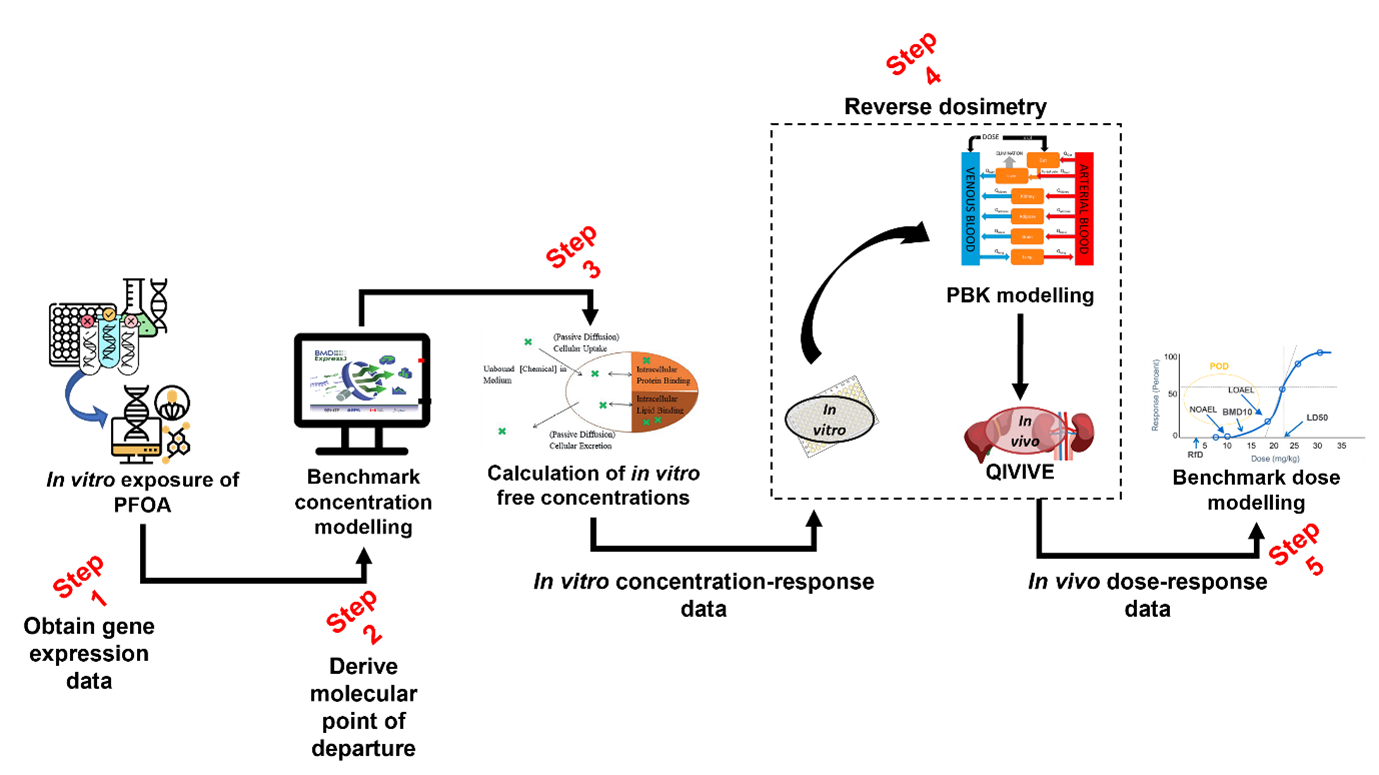
In silico workflow used to derive a health-based guidance value for PFOA. The image is multicoloured with black and red text. Each step of the flow has a miniature picture representing it with the step number written in red text. There are 5 steps:. 1: Obtain gene expression data. 2: Derive molecular point of departure. 3: Calculation of in vitro free concentrations. 4: Reverse dosimetry. 5: In vivo dose-response data.
Figure 5. In silico workflow used to derive a health-based guidance value for PFOA.
95. Data was generated in Step 1 (Figure 5) by exposing human liver spheroids to 10 different concentrations of four different PFASs and analysed over four time points: days 1, 4, 10, and 14 (Rowan-Carroll et al. 2021). The expression patterns of about 3000 toxicologically relevant/representative genes were then analysed for their effects in the toxicological assay. The in vitro effects of the PFAS known as perfluorooctanoic acid (PFOA) were modelled at day 10 of exposure, as it was the best time point to observe differentially expressed genes.
96. The BMD software BMDExpress3 Releases · auerbachs/BMDExpress-3 (github.com) (described in the section below) was employed in Step 2 (Figure 5) to derive molecular points of departure from the gene expression data obtained from the literature and Gene Expression Omnibus ( GEO Accession viewer (nih.gov). Modelling was performed under expert guidance. The BMD software provided, as an output, the chosen models for each gene as well as the model averaging for the benchmark concentration as well as both lower and upper bounds of the confidence interval.
97. In silico modelling of the toxicokinetic properties of PFOA is performed as part of the characterisation process using a calibrated model (Step 3 and 4, Figure 5). In the final step (Step 5) of the workflow, PROAST or alternatively, EFSA’s Bayesian BMD modelling suite, (EFSA - Sign in (b2clogin.com) was employed to derive a final health-based guidance value for PFOA using the in vivo dose-response data we had obtained from Step 3 and 4.
User experience
BMDExpress3
98. BMDExpress3 is a software tool designed for the benchmark dose analyses of genomic data. The software application is designed to perform a stepwise analysis to identify the subset of genes that demonstrate significant dose-response behaviour (Yang et al., 2007).
99. Before use, the software must be downloaded and installed onto the desktop (Releases · auerbachs/BMDExpress-3 (github.com). No account or sign up is required and step-by-step guidance on the setup and use of the software is available (How to Use the Application · auerbachs/BMDExpress-3 Wiki · GitHub ). The application has been developed significantly since its first release and software can be configured to look for the most up to date version available when starting each time to ensure the latest functionalities are available for the user.
Data Input
100. Gene expression data from human liver spheroids were analysed using BMDExpress3 and the dose response relationship analysed using the suite of in-built DRMs. The software can handle a range of data types; however, the data must be formatted correctly as the software only accepts tab delimited text files as input with correctly labelled columns and rows (see Figure 6). It was the users experience that log-transforming the data was preferable and recommended.
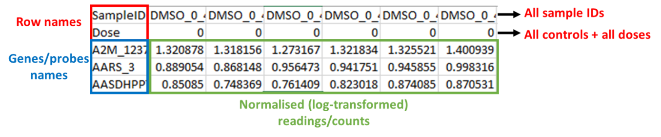
Example of formatted input data for BMDExpress3. Figure 6 shows a table of data with labels. The table has black text. Cells are outlined in red, blue, green and black. The table is labelled in different coloured text, blue red, green and black. On the right side of the table next to the top row are 2 black arrows pointing right with red text next to them. The red text reads: All Sample ID's and All controls+ all doses. The labels of the table are: Red top left: Row names. Blue bottom left: Genes/probes names. Green bottom centre: Normalised (log - transformed) readings/counts.
Figure 6. Example of formatted input data for BMDExpress3. Files must be saved as tab delimited excel files and the columns must be arranged as shown in the figure. The first row contains SampleIDs, the second row contains assigned dose (or concentration) levels, and all probes/genes/ metabolites are contianed in the third row onwards. Readings/counts must be normalised (log-transformed) before entry.
101. After preparing the data to import into BMDExpress3, the user can select the most appropriate platform for their data, as the software recognises some of the most used formats available. For this study, the appropriate platform was “BioSpyder S1500_Plus_Plus_Human_2.0 191113”.
Model Selection and operation
102. All of the dose-response curve fit models utilized by BMDExpress are those contained within USEPA BMDS software (Benchmark Dose Tools | US EPA). US EPA, 2022). A full discussion of these models is provided in Annex B. The user can select Power, Exponential, Hill and Linear models. The user can set the benchmark response to be a percentage or standard deviation when compared to controls and there is a graphical user interface and accompanying tutorial available showing how to work with dose- and concentration-response data (Benchmark Dose Analysis · auerbachs/BMDExpress-3 Wiki · GitHub).
103. The BMDExpress software also allows the option to flag Hill Models with ‘k’ Parameter < [selected value]. This allows the user to specify that if the Hill model is selected as one of the models to fit the data, it will be flagged if its ‘k’ parameter is smaller than the lowest positive dose, or a fraction (1/2, or 1/3) of the lowest positive dose (Annex B). As discussed in “Constraining or not constraining the models” section above, this option is included since the Hill model may provide unrealistic BMD and BMDL values for certain dose response curves, even when it provides the lowest AIC value. Once flagged the user can then choose a range of options including whether to include or exclude the flagged model or models from the final analysis.
104. When analysing the results, the user can filter data using their set of criteria; in this case study the following rules were used to ensure minimised uncertainty and maximise the confidence in the identification of genes exhibiting concentration-response relationships:
Custom settings employed in this study were as follows:
- ·K < 1/3, to flag Hill models
- BMR (benchmark response) = 1 SD
- 250 iterations
- Post-modelling filters to exclude low quality data:
§ Data were excluded if the BMD > highest concentration of test compound used in the in vitro experiments.
§ Data were excluded if the BMDU/BMDL ≥ 40 (as this indicated a high degree of uncertainty about the BMD and resulting RP.
§ Data were excluded if the p < 0.1.
Data output and visualisation
105. The main screen of BMDExpress3 interface displays the assembled BMD analysis result for all genes modelled. The user has a range of options to interact with the results table and customise visualisation e.g., toggling columns on/off, adding filter criteria, marking selected data, and selecting or creating their charts to represent the data (Figure 7). The results can be readily exported as a tab delimited file that is compatible with other spreadsheet editors (MS Excel, LibreOffice Calc, etc.).
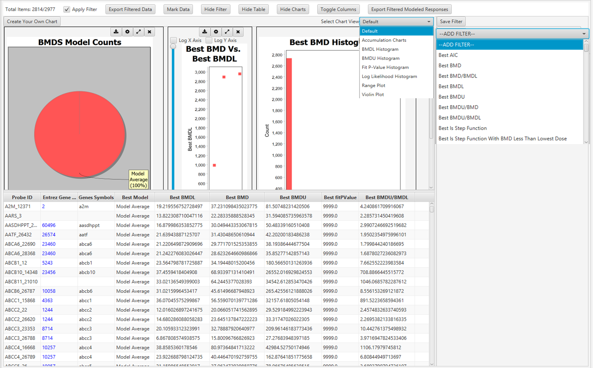
Graphical user interface of BMDExpress3 showing BMD analysis. The figure shows a screenshot of the programme in use.
Figure 7. Graphical user interface of BMDExpress3 showing BMD analysis. Each row represents a Probe ID that was previously imported into the software (see Figure 6).
106. Each row (“Entrez Gene ID") on the main screen (Figure 7) is clickable and will open a new window named “Curve Viewer” (Figure 8). The Curve Viewer interface provides both visual and numerical outputs for the BMD modelling operation. Users are provided with a plot of the experimental data and superimposed model fits along with the model average. The user can choose to open a drop-down list and select other available models to inspect their respective plots. Likewise, the user can click over the Probe ID (ECH1_2022) to open a drop-down list and access other Probes (experimental data sets) to inspect their models and plots. The chart can be edited (title, axis labels, font type and size, colours, etc) and can be exported as an image (.jpg, .png, and .svg).
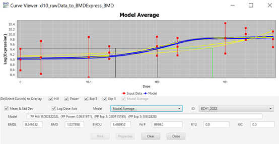
Curve viewer window of BMDExpress3. This figure shows a screen shot of the Curve viewer window. It displays a graph and the associated parameters chosen to create it.
Figure 8. Curve viewer window of BMDExpress3. The software allows the visualisation of dose-response data and fitted models alongside the estimated BMD model parameter and weights. Users have the option to select individual models or the model average, as well as visualizing the different experimental data sets.
PROAST
107. PROAST is a software package for the statistical analysis of dose-response data. Its main purpose is dose-response modelling of toxicological data. PROAST was operated online, where all the features can be easily accessed after creating a free account to be registered as a user EFSA - Sign in (b2clogin.com).
Data Input
108. Unlike BMDExpress3, PROAST allows the user to either input a tab delimited text file or a comma separated text file. There is no predesignated column format; the user selects the column corresponding to the test compound concentrations and the column corresponding to the response variables. It is necessary for the user to select the correct column with the responses and the type of response (quantal, binary, or continuous) along with the type of data (individual or summary). There is also the ability to add (or not) a litter effect if required.
Model Selection and operation
109. In the “Fit models” tab, the user can select the independent variable (dose) and the response variable(s), as well as add covariates if that is necessary, along with the choice of models and whether model averaging will be applied. The user can select how many bootstraps will be performed, with the default value set at 200. The maximum difference in AIC for model acceptance is 2 by default, but the user can change this value too.
110. The benchmark response (BMR), shown in the PROAST software as critical effect size (CES), is set as 0.05 or 5% as the default value but this can be altered to whatever the user decides. The user can also select the confidence level for the BMD confidence intervals (upper and lower bounds) with the default value set at 0.9 or 90%. In the present study, these parameters were left set at their default values.
Data output and visualisation
111. Once the models are fit, a report with all standard plots can be downloaded or the user can generate personalised plots according to their needs (Figure 9). The online version of the results is displayed on screen as well, and information about the BMD values and the best model(s), as well as the weights for the model averaging are provided alongside the model summaries (not shown).
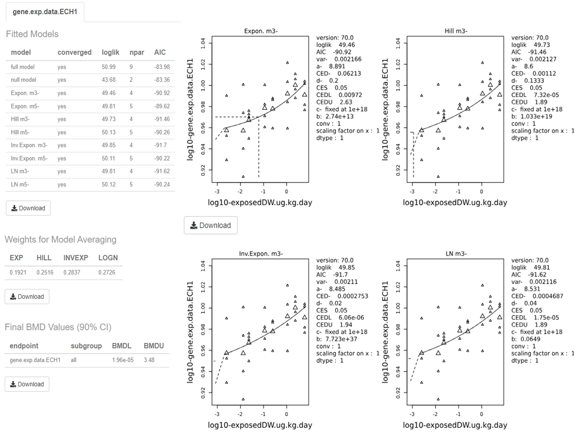
Output screen of PROAST web application. The figure shows a screen shot of the output from the application. It is made up pf multiple graphs and tables.
Figure 9. Output screen of PROAST web application. The software visualises the dose-response data along with the fitted BMD models. The estimated BMD model parameters are shown to the right of the graphs. Users can download each image and table individually by clicking on their respective “Download” button.
112. The visualised output displays the plots alongside the calculated BMD, BMDL, and BMDU (In the software these are displayed as the critical effect dose, CED, critical effect dose lower bound, CEDL, and critical effect dose upper bound, CEDU, respectively). Note: The standard plots display data on a log10 scale. Users need to be aware that the data presented beside the plot is dependent upon the units that were input by the user initially. The page also displays the plotted bootstrap models (Default: 200) with the averaged BMDL, BMDU, and the confidence intervals.
PROAST Bayesian BMD modelling
113. EFSA also offers a web application for Bayesian BMD modelling (EFSA - Sign in (b2clogin.com). The rational and mathematical basis to the Bayesian BMD approach is discussed in detail in EFSA’s 2022 updated BMD guidance and practical demonstration of the software and additional background is also available in the form of the publicly available video of the 2023 EFSA BMD workshop (EFSA, 2022; EFSA Workshop, 2023).
Data Input
114. The data input format is the same as that required by PROAST – tab or comma delimited text file with dose-response data.
Model Selection and operation
115. The user can check if their data is suitable and of sufficient quality for dose-response modelling. The software implements an initial analysis of the dose response data to determine if there is sufficient evidence for a substantial dose-effect before the full modelling is attempted.
116. The distribution can be selected as normal or log-normal, as appropriate and users can decide whether to perform a sensitivity analysis or not. As with the non-Bayesian software, the user can define CES (aka BMR) and the credible interval. Additionally, the user can select whether the Prior information is set to a default (uninformative) prior or if an informative prior is to be used. This allows the user to add additional information to the modelling from outside the experimental data set, such as information from historical experiments which will then be used to calculate the posterior likelihood distribution.
117. The Bayesian BMD web application also allows the user to access advanced settings which allows them to choose for example:
- The type of sampling method (Laplace or Bridge) employed. (Note: The Laplace method uses approximations to derive the sampling data, however Bridge sampling is more computationally expensive)
- Whether to extend (or not) the dosing range beyond the range of the experimental data
- Which models to include - Up to 16 different models are available. (Available models are discussed in EFSA, 2022 updated BMD Guidance (included as part of Annex B).
- The Number of draws to be made from posterior sampling: The Number of Markov chain Monte Carlo (MCMC) chains and the Number of MCMC interactions as well as how many MCMC interactions should be discarded as warmup.
Data output and visualisation
118. Once the models are fit, the Bayesian BMD application displays the results on-screen, plotting the results of the modelling alongside the experimental data. The posterior distribution, along with the 90% confidence intervals are superimposed on the same graph by default (Figure 10). An advanced plotting option is also available, for personalised, higher quality plots/images.
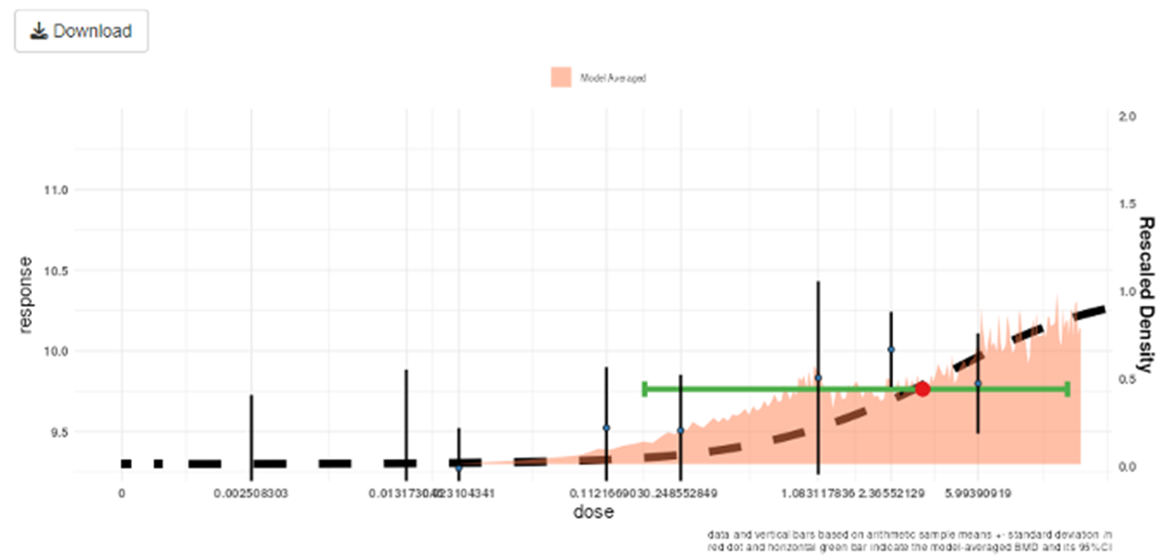
Output of Bayesian BMD web application. The figure shows a graph. The graph is multicoloured with black text labels.
Figure 10. Output of the Bayesian BMD web application. Vertical lines show the observed mean responses ± standard deviation of experimental data. The dashed curve is a fitted dose-response model. The density region shows the posterior distribution of the BMD and the green line indicates the boundaries of the two-sided 90% credible interval of the BMD. The BMDL, is the 95% one-sided lower bound of the credible interval for the BMD. Similarly, the BMDU is the 95% one-sided upper bound of the 90% credible interval for the BMD.
119. The software also provides a breakdown of the individual models in the form of a table along with their BMDs, BMDLs, BMDUs, and the weights that the software accorded to each one. The user can also download an automatically generated report by clicking the “Download report” button available in the top left corner of the webpage (Figure 11).
120. Finally, the model averaged results for the BMD, BMDL, BMDU are presented in a separate table along with a notification if any of the constituent models defy the normality assumptions (green indicated no normality tests have been rejected for any model).
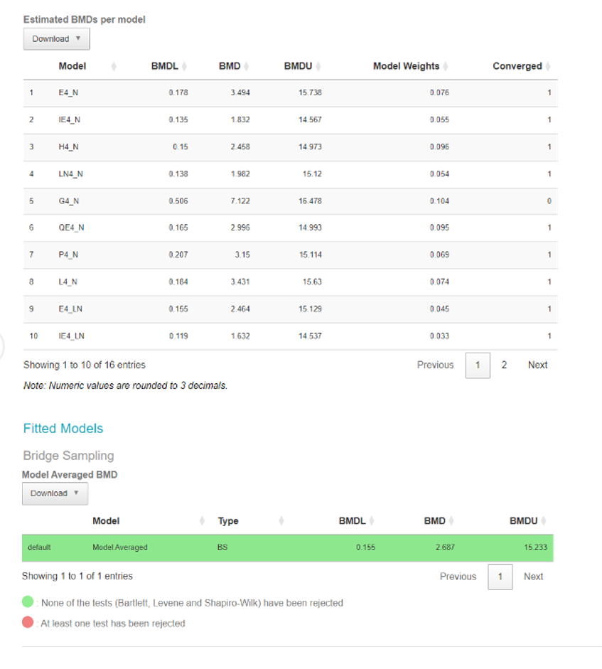
Output screen of Bayesian BMD web application. This figure shows an output screenshot from the application. It shows the results from the data tested. The results are coloured green or red. Green = None of the tests have been rejected. Red= At least one test has been rejected.
Figure 11. Output screen of the Bayesian BMD web application. Tables showing the BMDs, BMDLs, BMDUs, for the various individual fitted models (Upper table) or Model averaged curve (Lower table).
Table 1. User generated feedback on the three BMD modelling platforms used in this study.
|
Details |
BMDExpress3 |
EFSA / PROAST |
EFSA Bayesian BMD modelling |
|
Platform and operations. |
Standalone software (Installation Required). |
Web application (no need to download and install). |
Web application (no need to download and install). |
|
Account required. |
No |
Yes |
Yes |
|
First use / Learning curve. |
Easy to get started. |
Easy to get started. |
Easy to get started. |
|
Training or Online material available? |
How to setup and use webpage - Very useful and instructive Benchmark Dose Analysis · auerbachs/BMDExpress-3 Wiki · GitHub. Wiki page is extremely useful, rich in screenshots of the application, and the video tutorials are a great plus Benchmark Dose Analysis · auerbachs/BMDExpress-3 Wiki · GitHub. |
Training was primarily from other expert users. |
Training was primarily from other expert users. |
|
File format accepted for data input. |
Only accepts tab delimited text files. File needs to be formatted in specific way (name on columns and rows). |
Tab delimited text file or a comma separated text file, can deal with both.
|
Tab delimited text file or a comma separated text file, can deal with both.
|
|
Continuous data accepted? |
Yes
|
Yes
|
Yes
|
|
Nested continuous data accepted? (e.g. litter effects). |
No |
Yes
|
Yes
|
|
Quantal data accepted? |
No |
Yes
|
Yes
|
|
Suitability for biological analysis. |
Better for analysing ‘omics data (genes and metabolites), Less practical for other data types (such as clinical chemistry or exposure data) BMDExpress3 requires extra steps for formatting the data and selecting “generic platform” is |
Flexible software which can handle a range of data types.
|
Flexible software which can handle a range of data types.
|
No Detail. |
A must prior to modelling. |
No Detail. |
No detail. |
|
User interface.
|
Graphical User Interface (GUI).
|
Both R version (command line) and web application with GUI possible. |
Web application with (GUI).
|
|
Range of Models available. |
Dose-response models utilized by are those contained within USEPA BMDS software (www.epa.gov/bmds, See Annex B for full discussion.). Users can choose from a range of models: Hill, Power, Exponential (3 and 5), Linear, and Polynomial (2, 3, and 4). As an additional option for modelling, there is also GCurveP (Sciome). |
Automatically generates: · Hill, · Exponential, · Lognormal, · Inverse Exponential
See Annex B for full discussion. |
Users can choose from a range of 16 models:
Exponential Normal, Inverse Exponential Normal, Hill Normal, Lognormal Normal, Gamma Normal, Quadratic Exponential Normal, Probit Normal, Logit Normal, and their 8 Lognormal equivalents. See Annex B for full discussion. |
|
Model averaging Available? |
Model averaging Available? |
Model averaging Available? |
Model averaging Available? |
|
Details. |
Yes, User can select Hill, Power, and Exponential (3 and 5) models to run the model averaging module.
|
Yes, The possibility of visualization of the weights for each model in PROAST is an advantage.
|
Yes, User can select 16 different models and two different sampling methods, as well as visualize the weights for each model in Bayesian BMD. |
|
Includes covariates analysis? |
No |
Yes |
Yes |
|
Bayesian analysis. |
MCMC Bayesian approaches to model averaging (available in v.3, with ToxicR functionality). |
No |
Yes |
|
Option to email user when modelling is complete? |
No |
Yes |
Yes |
|
Graphical output. |
Visual plot of the data and BMD curves.
Limited plot editing capabilities: Software allows for the modifications of axis names but only.original scales for y-axis and x-axis. |
Visual plot of the data and BMD curves.
Includes more options to modify output graphs, change scales etc. (e.g. log-scales). Advanced plotting features allows publication quality images to be produced and downloaded easily. |
Visual plot of the data and BMD curves.
Includes more options to modify output graphs, change scales etc. (e.g. log-scales). Advanced plotting features allows publication quality images to be produced and downloaded easily. |
|
Automatically generate final reports? |
No |
Yes
|
Yes
|
|
Available online at:
|
Version 3 is available at: Releases · auerbachs/BMDExpress-3 (github.com). Version 2 command line is available at: Command Line · auerbachs/BMDExpress-3 Wiki · GitHub along with instructions on how to use it. |
Conclusions
121. Traditionally, the NOAEL approach has been used for developing toxicological “safe dose” estimates such as reference doses (RfDs), acceptable daily intake (ADIs) values, or other values that can be used as HBGVs for chemical risk assessments. However, BMD modelling is now considered the preferred approach for deriving RPs for developing these “safe dose” estimates. BMD modelling allows a more quantitative and informative estimate of these RPs than the NOAEL approach.
122. Ideally, the BMD model used would be one that mimics the behaviour of the underlying biological system. However, in practice, most of the time the BMD modelling approach is an attempt to find the “best” mathematical model that describes the data, from a range of potential mathematical models.
123. The choice of model or models is determined by the nature of the data making up the endpoint of interest, the experimental design, dose selection etc. Similarly, the BMR can be selected based on toxicological and statistical consideration. However, in the absence of information about what biological response may be considered “adverse”, EFSA recommend either a BMR of 5% (continuous) or 10% (quantal) be set as a default depending on the data type. In contrast, the EPA recommend the BMR for continuous data be set in terms of a change relative to the standard deviation of the data, rather than % response, but agree that a BMR of 10% for quantal data is appropriate.
124. Historically, BMD software for DRMs used frequentist methodologies. However, developments in BMD software have made possible the use of Bayesian methods for the same approach. EFSA now recommend the Bayesian approach as the preferred approach to BMD modelling.
125. The BMD approach can be applied to all chemicals in food, independent of the nature or source. The BMD approach can be applied to a range of data types in including classical in vitro toxicological data, but also gene expression data, and even epidemiological data.
Advantages
126. Both EFSA and the US EPA consider the BMD approach to be the more quantitative and more scientifically advanced approach to deriving the RP from dose response data, compared to the NOAEL approach.
127. The BMD approach uses all the available dose-response information within a given dataset. The NOAEL approach, in contrast, effectively uses only the data that make up the control group and one other dose group.
128. The BMD approach provides important information regarding the uncertainties in the data. The output of the BMD approach provides a quantitative assessment of data quality, as described by the confidence (or credible) intervals.
129. BMD software can be developed and tailored to the needs of researchers. For example, specialist BMD modelling software, such as BMDExpress3 have been developed to meet the specifics of dose-response gene expression data.
130. BMD software is publicly available and accessible, along with guidance documents, user manuals tutorial videos and workshop recordings.
Challenges
131. BMD modelling software may require some training to use. Different software packages would require separate training to provide competence.
132. There are notable areas of divergence in the guidance provided by organisations such as the US EPA and EFSA with regards to BMD use and its best practices.
133. There are still significant differences in the operation and statistical basis for the various BMD modelling software. This means, in practice, that two different software analysing the same data, may generate potentially different BMD and BMDL values, and consequently will generate two different RPs and HBGVs.
Recommendations.
134. Training and competency workshops would be valuable to provide practical training for anyone on the COT or in the FSA interested in using BMD modelling approaches and BMD software.
135. Considering the areas of divergence in the current guidance around BMD, greater clarity on the accepted best practices would be appropriate. Further attempts to harmonise the approach to BMD modelling across agencies, governments and regulators would also be desirable.
136. Communication with industry, regulators and expert groups should also be encouraged to ensure that BMD modelling is adopted and integrated appropriately within the broader regulatory chemical safety environment. Development of an OECD (Organisation for Economic Co-operation and Development) guideline, as well as government and regulatory guidance around BMD implementation and experimental design, as well as clarity on requirements, reporting templates etc., should be considered.
137. A review of BMD modelling in chemical risk assessment, within an appropriate timeframe in the future, is recommended, particularly considering the rapidly changing computational and technological landscape.
Questions on which the views of the Committee are sought:
i) Does the report capture the most up to date information and details on benchmark dose modelling?
ii) Are the Members content with the areas covered in the report?
iii) Can the available BMD guidance and resources support the integration of new approach methodologies in future guidance?
iv) Can BMD modelling provide a useful and practical tool that can be applied in a chemical risk assessment?
v) Do Members have any examples of when this approach could be applied and or recommendations?
Do the Members have any other comments?
Secretariat
February 2024
List of Abbreviations
|
ADI |
Acceptable Daily Intake |
|
AIC |
Akaike Information Criterion |
|
BMA |
Bayesian Model Averaging |
|
BMD |
Benchmark Dose |
|
BMDL |
Benchmark Dose lower bound |
|
BMDS |
Benchmark Dose Software |
|
BMDU |
Benchmark Dose upper bound |
|
BMR |
Benchmark response |
|
CED |
Critical Effect Dose |
|
CEDL |
Critical Effect Dose lower bound |
|
CEDU |
Critical Effect Dose upper bound |
|
CES |
Critical Effect Size |
|
COC |
The Committee on Carcinogenicity of Chemicals in Food, Consumer Products and the Environment |
|
COM |
The Committee on Mutagenicity of Chemicals in Food, Consumer Products and the Environment |
|
COT |
The Committee on the Toxicity of Chemicals in Food, Consumer Products and the Environment |
|
DRM |
Dose-Response Models |
|
EFSA |
European Food Safety Authority |
|
FAO |
Food and Agriculture Organization |
|
FSA |
Food Standards Agency |
|
HBGV |
Health Based Guidance Values |
|
IPCS |
International Programme on Chemical Safety |
|
IRIS |
Integrated Risk Information System |
|
JECFA |
Joint FAO/WHO Expert Committee on Food Additives |
|
JMPR |
Joint FAO/WHO Meeting on Pesticide Residues |
|
LMS |
Linearised Multistage (model) |
|
LOAEL |
Lowest Observed Adverse Effect Level |
|
LVM |
Latent variable model |
|
MCMC |
Markov Chain Monte Carlo |
|
MLE |
Maximum-Likelihood Estimation |
|
MOE |
Margin of Exposure |
|
NOAEL |
No Observed Adverse Effect Level |
|
OECD |
Organisation for Economic Co-operation and Development |
|
OGD |
Other Government Departments |
|
PoD |
Point of Departure |
|
RfD |
Reference Dose |
|
RPF |
Relative Potency Factors |
|
SC |
Scientific Committee |
|
TEF |
Toxic Equivalency Factors |
|
UF |
Uncertainty Factor |
|
US EPA |
United States Environmental Protection Agency |
|
US NTP |
United States National Toxicology Program |
|
WHO |
World Health Organisation |
Technical terms
Bayesian: Statistical methodological approach that assigns probabilities or distributions to parameters based on prior data and applies Bayes’ theorem to revise the probabilities and distributions after obtaining the experimental data.
Bernoulli distribution: A discrete distribution having two possible outcomes: n=0 and n=1, where n=1 ("occurs") occurs with probability p and n=0 ("does not occur") occurs with probability q=1-p, where 0<p<1. In chemical toxicology, such a distribution might describe the probability of a discrete adverse outcome such as animal death or present of tumours i.e. it occurs or does not occur.
Bootstrap: A statistical technique based on multiple resampling. In a bootstrap approach, a probability distribution estimated from observed values is used to generate new samples. For example, based on a random sample of 20 data points in an experiment, the data might be resampled 1,000 times, calculating a standard deviation and a mean each time. The resulting distribution of some quantity of interest (e.g., the standard deviation or the mean) is used to calculate confidence limits or perform statistical tests in computationally complex situations, or where a particular distribution of an estimate or test statistic cannot be assumed.
Categorical Data: Data recorded in categories, either without a natural ordering (sex: male or female), or naturally ordered (ordinal, e.g., mild, moderate, or severe).
Confidence Interval: A statistically derived interval (typically consisting of lower and upper bounds) that has a specified probability of containing the true value of some estimated parameter, if the same population is sampled repeatedly. The interval is expected to include the true value of the estimated parameter with a specified confidence, e.g., 95%.
Convergence: In the case of a parameter estimate, approach to a single value with increasing number of computational iterations.
Covariate: An independent variable other than dose that may influence the effect of interest, e.g., age, body weight, sex.
Continuous Data: Data measured on a continuum, e.g., organ weight or blood biomarker concentration.
Coverage (in reference to Confidence Interval): The actual (as opposed to theoretical) probability that a population parameter is bounded by the limits of a given confidence interval procedure.
Dichotomise: The process of dividing or classifying objects, data, or events into two groups. For example, 50 animals could be classified into two groups, according to whether their weight exceeds some specified value.
Dichotomous Data (also known as Quantal Data): Type of data where an effect may be classified into one of two possible outcomes, e.g., dead or alive, with or without incidence of a specific symptom (e.g., tumour).
Dose-Response Model: A mathematical function that relates or predicts the occurrence or severity of an adverse effect to a given range of doses.
Extra Risk: A measure of the increase in risk of an adverse effect adjusted for the background incidence for the same effect. Extra risk is calculated as follows: [P(d)–P(0)] / [1–P(0)], where P = the probability of an effect and d = dose.
Frank Effect: An obvious or overtly clinically apparent toxic effect.
Goodness-of-Fit Statistic: A statistic that measures the deviation of observed data from predicted or hypothesized values. Some goodness-of-fit statistics can be used in statistical hypothesis tests, leading to rejection (or failure to reject) a model due to lack of an adequate fit.
Log Transformation: The process of taking logarithms of the data. Log transformations are often applied to continuous response data to make the transformed responses satisfy a normality assumption, if the data are lognormally distributed.
Margin of Exposure (MOE): Ratio of a dose that produces a specified effect, to an expected human dose.
Markov chain Monte Carlo (sampling): Markov Chain Monte Carlo sampling provides a class of algorithms for systematic random sampling from high-dimensional probability distributions. Unlike Monte Carlo sampling methods that are able to draw independent samples from a distribution, Markov Chain Monte Carlo methods draw samples where the next sample is dependent on the existing sample, called a Markov Chain.
Ordinal Data: see Categorical Data
Point of Departure (PoD): The point where the dose response curve moves away from background. It can be used as a basis for the setting of health-based exposure limits.
Probability Distribution: A statistical description (in the form of a distribution) of the relative probabilities of all possible outcomes of an event.
Quantal Data: see Dichotomous Data
Reference Dose (RfD): An estimate of a daily exposure to the human population (including sensitive subpopulations) that is likely to be without an appreciable risk of deleterious effects during a lifetime.
Reference point (RP): see Point of Departure.
Supralinear dose response: A dose-response relationship that is proportionately steepest at the lowest levels of exposure.
Uncertainty Factor (UF): A numerical value (often a factor of 3 or 10) used to adjust a NOAEL, LOAEL, or benchmark dose to derive a reference dose. Reasons for UFs to be applied as needed are to account for e.g., extrapolation of results in experimental animals to humans, interindividual variability (including sensitive subgroups), extrapolation from a LOAEL to a NOAEL, extrapolation of results from subchronic exposures to chronic exposures, and/or database inadequacies.
Variance: The variance in an experimental measurement remaining after accounting for variance due to the independent variables, e.g., dose, exposure duration, and age.
References
Akaike, H., 1973. Information theory and an extension of the maximum likelihood principle., in: Proceedings of the Second International Symposium on Information Theory. Akademiai Kiado, Budapest, Hungary, pp. 267–281.
Bokkers, B.G.H., Slob, W., 2007. Deriving a data-based interspecies assessment factor using the NOAEL and the benchmark dose approach. Crit Rev Toxicol 37, 355–373.
Bosgra, S., van der Voet, H., Boon, P.E., Slob, W., 2009. An integrated probabilistic framework for cumulative risk assessment of common mechanism chemicals in food: an example with organophosphorus pesticides. Regul Toxicol Pharmacol 54, 124–133.
Burnham, K.P., Anderson, D.R., 2004. Multimodel Inference: Understanding AIC and BIC in Model Selection. Sociological Methods & Research 33, 261–304.
Clyde, M.A., 2003. Model Averaging (Chapter) In S. J. Press (Ed.), Subjective and Objective Bayesian Statistics: Principles, Models, and Applications. John Wiley & Sons.
COT, 2020. The Committee on Toxicity of Chemicals in Food, Consumer Products and the Environment: Assessing chemical risks in food. Available at: Assessing chemical risks in food | Committee on Toxicity
Crump, K.S., 1984. A new method for determining allowable daily intakes. Fundam Appl Toxicol 4, 854–871.
Dekkers, S., de Heer, C., Rennen, M.A.J., 2001. Critical effect sizes in toxicological risk assessment: a comprehensive and critical evaluation. Environmental Toxicology and Pharmacology 10, 33–52.
EFSA, 2022. Guidance on the use of the benchmark dose approach in risk assessment. EFSA Journal 20, e07584. Available at: Guidance on the use of the benchmark dose approach in risk assessment | EFSA (europa.eu)
EFSA, 2017. Update: use of the benchmark dose approach in risk assessment. EFSA Journal 15, e04658. Available at: Update: use of the benchmark dose approach in risk assessment - - 2017 - EFSA Journal - Wiley Online Library
EFSA, 2009. Guidance of the Scientific Committee on Use of the benchmark dose approach in risk assessment. EFSA Journal 7, 1150. Available at: Guidance of the Scientific Committee on Use of the benchmark dose approach in risk assessment - - 2009 - EFSA Journal - Wiley Online Library
EFSA, 2005. Opinion of the Scientific Committee on a request from EFSA related to A Harmonised Approach for Risk Assessment of Substances Which are both Genotoxic and Carcinogenic. EFSA Journal 3, 282. Available at: Opinion of the Scientific Committee on a request from EFSA related to A Harmonised Approach for Risk Assessment of Substances Which are both Genotoxic and Carcinogenic (wiley.com)
EFSA Workshop, 2023. Workshop on EFSA’s updated Guidance on the use of the benchmark dose approach in risk assessment. Available at: Workshop on EFSA’s updated Guidance on the use of the benchmark dose approach in risk assessment | EFSA (europa.eu)
FAO/WHO, 2020. Principles and methods for the risk assessment of chemicals in food Environmental health criteria (240) Chapter 5 : Dose-Response Assessment and Derivation of Health-Based Guidance Values. Available at: chapter5-dose-response.pdf (who.int)
FAO/WHO, 2006. Safety evaluation of certain contaminants in food / prepared by the sixty-fourth meeting of the Joint FAO/WHO Expert Committee on Food Additives. WHO Food additives series; 55. Available at: Safety evaluation of certain contaminants in food / prepared by the sixty-fourth meeting of the Joint FAO/WHO Expert Committee on Food Additives
FAO/WHO, 2005. International Programme on Chemical Safety, Principles for Modelling Dose-Response for the Risk Assessment of Chemicals. Environmental health criteria; 239. Geneva, World Health Organization. Available at: Environmental Health Criteria 239: PRINCIPLES FOR MODELLING DOSE–RESPONSE FOR THE RISK ASSESSMENT OF CHEMICALS (inchem.org)
FAO/WHO, 1990. International Programme on Chemical Safety. Environmental Health Criteria 104: Principles for the toxicological assessment of pesticide residues in food. Geneva, Switzerland, World Health Organization. Available at: Pesticide residues in food, principles for the toxicological assessment of (EHC 104, 1990) (inchem.org)
Gehlhaus, M.W., Gift, J.S., Hogan, K.A., Kopylev, L., Schlosser, P.M., Kadry, A.-R., 2011. Approaches to cancer assessment in EPA’s Integrated Risk Information System. Toxicol Appl Pharmacol 254, 170–180.
Gephart, L.A., Salminen, W.F., Nicolich, M.J., Pelekis, M., 2001. Evaluation of Subchronic Toxicity Data Using the Benchmark Dose Approach. Regulatory Toxicology and Pharmacology 33, 37–59.
Haber, L.T., Dourson, M.L., Allen, B.C., Hertzberg, R.C., Parker, A., Vincent, M.J., Maier, A., Boobis, A.R., 2018. Benchmark dose (BMD) modeling: current practice, issues, and challenges. Crit Rev Toxicol 48, 387–415.
Ji, C., Weissmann, A., Shao, K., 2022. A computational system for Bayesian benchmark dose estimation of genomic data in BBMD. Environ Int 161,
Kang, S.H., Kodell, R.L., Chen, J.J., 2000. Incorporating model uncertainties along with data uncertainties in microbial risk assessment. Regul Toxicol Pharmacol 32, 68–72.
Kavlock, R.J., Allen, B.C., Faustman, E.M., Kimmel, C.A., 1995. Dose-response assessments for developmental toxicity. IV. Benchmark doses for fetal weight changes. Fundam Appl Toxicol 26, 211–222.
Shao, K., Gift, J.S., 2014. Model Uncertainty and Bayesian Model Averaged Benchmark Dose Estimation for Continuous Data. Risk Anal 34, 101–120.
Shao, K., Shapiro, A.J., 2018. A Web-Based System for Bayesian Benchmark Dose Estimation. Environ Health Perspect 126, 017002.
Slob, W., 2014. Benchmark dose and the three Rs. Part I. Getting more information from the same number of animals. Critical Reviews in Toxicology 44, 557–567.
Slob, W., 2002. Dose-Response Modeling of Continuous Endpoints. Toxicological Sciences 66, 298–312.
Slob, W., Setzer, R.W., 2014. Shape and steepness of toxicological dose-response relationships of continuous endpoints. Crit Rev Toxicol 44, 270–297.
US EPA, 2022. Benchmark Dose Software User Guide Version 3.3. Available at: BMDS Version 3.3 User Guide (Oct 2022) | Benchmark Dose Software (BMDS) | US EPA
US EPA, 2017. United States Environmental Protection Agency. Categorical Regression (CatReg) User Guide (Version 3.0.1.7). Available at: CatReg 3.1 User Guide (epa.gov)
US EPA, 2012. Benchmark Dose Technical Guidance. Available at: benchmark dose technical guidance (epa.gov)
Wheeler, M.W., Bailer, A.J., 2009. Comparing model averaging with other model selection strategies for benchmark dose estimation. Environ Ecol Stat 16, 37–51.
Wheeler, M.W., Bailer, A.J., 2008. Model Averaging Software for Dichotomous Dose Response Risk Estimation. Journal of Statistical Software 26, 1–15.
Wheeler, M.W., Bailer, A.J., 2007. Properties of Model-Averaged BMDLs: A Study of Model Averaging in Dichotomous Response Risk Estimation. Risk Analysis 27, 659–670.
Yang, L., Allen, B.C., Thomas, R.S., 2007. BMDExpress: a software tool for the benchmark dose analyses of genomic data. BMC Genomics 8, 387.
TOX/2024/03 Annex A
Benchmark Dose Models included in BMDS and PROAST
1. Most of the models in the following tables were developed by U.S. EPA and RIVM National Institute for Public Health and the Environment and are available in BMDS and PROAST, unless otherwise noted.
2. The current models and mathematical descriptions appear as in the most recent documentation: Benchmark Dose Software (BMDS) Version 3.3 User Guide, U.S. EPA, published October 2022, and EFSA’s Guidance on the use of the benchmark dose approach in risk assessment, published in 2017 and 2022. Models no longer available, but that appear in previous documentation or versions of the software are not considered here but are discussed in the relevant publication.
Note: For copyright reasons the papers in the Annexes are not included in the published version on the COT website. The bibliographic details of the annexed material are listed above. The documents are all in the public domain and individuals can obtain them by application to appropriate sources.
Table 1. List of Continuous and Dichotomous Models available
|
List of Continuous models |
BMDS Version 3.3 |
PROAST (EFSA 2017) |
PROAST (EFSA 2022) |
|
Exponential |
Yes |
Yes |
Yes |
|
Inverse Exponential |
No |
No |
Yes |
|
Hill |
Yes |
Yes |
Yes |
|
Linear |
Yes |
No |
No |
|
Polynomial Power |
Yes |
No |
No |
|
Gamma |
No |
No |
Yes |
|
LMS Two-stage |
No |
No |
Yes |
|
Probit |
No |
No |
Yes |
|
Logistic |
No |
No |
Yes |
|
List of Dichotomous models |
BMDS Version 3.3 |
PROAST (EFSA 2017) |
PROAST (EFSA 2022) |
|
Exponential |
No |
No |
Yes |
|
Inverse Exponential |
No |
No |
Yes |
|
Hill |
No |
No |
Yes |
|
LMS Two-stage |
No |
Yes |
Yes |
|
Gamma |
Yes |
Yes |
Yes |
|
Logistic |
Yes |
Yes |
Yes |
|
Log-Logistic |
Yes |
Yes |
No |
|
Log Probit |
Yes |
Yes |
No |
|
Multistage |
Yes |
No |
No |
|
Probit |
Yes |
Yes |
Yes |
|
Weibull |
Yes |
Yes |
No |
|
Quantal Linear |
Yes |
No |
No |
|
Dichotomous Hill |
Yes |
No |
No |
|
Latent variable models (LVM) |
No |
Yes |
No |
|
Multi-tumor (MS_Combo) |
Yes |
No |
No |
|
List of Nested Dichotomous Models |
BMDS Version 3.3 |
PROAST (EFSA 2017) |
PROAST (EFSA 2022) |
|
Nested Logistic |
Yes |
|
No |
EFSA 2022 - Guidance on BMD approach in risk assessment.
3. The models in the following tables were described by EFSA in their 2022 guidance and are available as part of the PROAST BMD web application software. This section provides basic information about the statistical methodology and components of a single dose-response model for a single continuous endpoint. The relevant information has been reproduced here verbatim:
Dose–response model for a single continuous endpoint
Only two parametric distributions, which are fully characterised by their functional form and two parameters (central location and spread around the centre) are considered in this document: the normal distribution and the log-normal distribution. The normal distribution is symmetric, whereas the log-normal is a right-skewed distribution. They both share theoretical and computational advantages Guidance on BMD approach in risk assessment and have been proven to fit well to many biological endpoints (Johnson et al., 1994). As endpoints are assumed to be positive-valued, a left-skewed distribution is not considered. If empirical or biological evidence necessitates, other distributions (e.g., the inverse Gaussian distribution, the gamma distribution) may be considered suitable as well, but the extension of the statistical modelling framework, as described in this section, to other distributions is not straightforward, nor is its implementation in the BMD application hosted in the R4EU servers. Before modelling the central location of the normal and log-normal distribution as a function of dose, the relevant characteristics of both distributions are summarised below.
Modelling the distribution of the response
It is assumed that the observations of y, given a specified dose (denoted as j x), vary according to the normal distribution:
y|x ∼ N(μ(x), σ2)
where μ(x) represents the mean and σ2 the variance of the response at dose x. The normal distribution is a symmetric distribution (implying that μ(x) is the median as well). The true distribution of the response y is unknown, but the normal distribution is known to often be a good approximation for that true distribution, especially if it is a symmetric distribution, even if the endpoint is restricted to be positive. The distribution only shifts up or down according to the value of the mean μ(x), but the variance σ2 and the typical symmetric ‘bell shape’ of the distribution remains invariant to changes in dose.
In addition to the normal distribution, also the log-normal distribution can be considered:
y|x ∼ LOGN(μ(x), σ2)
This distribution is automatically restricted to positive values and is skewed to the right. Typically, the notation of the two parameters is identical to that of the two parameters of the normal distribution, but the interpretation is different. It holds that:
y|x ∼ LOGN(μ(x), σ2) ↔ log(y|x) ∼ N(μ(x), σ2)
implying that μ(x) and σ2 do not refer to the mean and the variance of the response itself but to the mean and the variance of the log-transformed response. Again, it is assumed that the parameter σ2 does not depend on dose. The characteristics on the original scale are shown in Table 1 for both distributions. Note that, although the parameter σ2 does not depend on dose, the variance of a log-normally distributed response does depend on dose, as it depends on the parameter μ(x) as well. For a log-normally distributed response, the coefficient of variation (standard deviation divided by mean) does not depend on dose (constant, with value eσ2-1 )
Modelling the central location of the distribution as a function of dose
Next to the specification of the distribution (normal or log-normal), a suite of eight candidate models for μ(x) is used, as shown in Table 2. All candidate models μ(x) share some basic properties P1-P4:
Basic properties (P1-P4)
P1: the median can only take positive values (e.g. a median organ weight cannot be ≤ 0), so.
- μ(x) > 0 if a normally distributed endpoint is considered;
- no constraint on values of μ(x) > 0 for a log-normally distributed endpoint;
P2: they are monotone increasing or decreasing, for both distributions;
P3: they are continuous functions of dose x, for both distributions;
P4: they reach a horizontal asymptote for very high dose levels (mathematically x = ∞), for both distributions, such that they are suitable for data that level off to a maximum response.
In the next paragraphs, three families of models (1a, 1b and 2) are introduced. All members of these families are flexible four-parameter non-linear models, and all share the basic properties P1–P4. The above-mentioned eight candidate models have been selected from these three families. This selection incorporates the familiar exponential and Hill model from the previous guidance (EFSA, 2017), and extends it with alternative flexible models leading to a unification of models across both type of endpoints, continuous or quantal. The model structure of Family 1a/b and Family 2 is fundamentally different. The general structure of Family 1a and 1b with the central role of the median background response and the maximum change in median response (parameters a and c) is identical, but the two other parameters b and d operate functionally differently in both subfamilies.
- Family 1a and 1b: all models for μð Þx have the following structure
μ(x) = a(1 + (c - 1) F(x; b, d)), b, d > 0,
for some particular but known function F, having the properties:
§ defined for x ≥ 0;
§ monotone increasing;
§ F(0; b, d) = 0 and F(∞; b, d) = 1 regardless the values of b and d.
For all members of Family 1a, the parameter d acts as a power xd , whereas it operates differently in Family 1b (see Table 2). The parameters a, b, c, d have a particular interpretation:
§ a = μ(0) is linked to the median background response;
§ c = μ(∞) / μ(0) is linked to the maximum change in median response, as compared to the background response; for c > 1 (resp. c < 1) the median response is monotone increasing (resp. decreasing) as a function of dose x;
§ b and d characterise the shape of change in response from median background response to maximum change in median response, via the identity:
F(x; b, d) = μx-μ(0) μ∞-μ(0) '
the model is reparametrised in terms of the parameter a, c (representing the background response and the maximum change in response), the BMD (the potency, see Table 2, and replacing the parameter b) and the parameter d.
- Family 2 increasing: increasing models for μð Þx from this family have the following structure:
μ(x) = cF(a + bxd), b, d > 0
for some particular but known function F, having the properties:
§ defined for any value of a + bxd;
§ monotone increasing;
§ F(-∞; b, d) = 0 and F(∞; b, d) = 1 regardless the values of b and d:
The parameters a, b, c, d have a particular interpretation:
§ c = μ(∞) and a = F-1 (μ(0) /μ(∞)) and determine the median background response and the maximum change in median response, as compared to the background response;
§ b and d characterise the shape of change in response from median background response to maximum change in median response, via the identity:
bxd = F-1 (μ(x) /μ(∞)) - F-1 (μ(0) /μ(∞)),
the model is reparametrised in terms of the parameter a, c (representing the background response and the maximum change in response), the BMD (the potency, see Table 2, and replacing the parameter b) and the parameter d.
- Family 2 decreasing: decreasing models for μð Þx from this family have the following structure:
μ(x) = a ((1 + F(c)) – F(c + bxd)), b,d > 0
for some particular but known function F, having the properties:
§ defined for all values of c and all values of c + bxd;
§ monotone increasing;
§ F(-∞; b, d) = 0 and F(∞; b, d) = 1 regardless the values of b and d:
The parameters a, b, c, d have a particular interpretation:
§ a = μ(x) and c = F-1 (μ(∞) /μ(0)) determine the median background response and the maximum change in median response, as compared to the background response;
§ b and d characterise the shape of change in response from median background response to maximum change in median response, via the identity:
bxd = F-1 (μ(∞)/μ(0) - (μ(x)/ - (μ(0))/(μ(0)) - F-1 (μ(∞)/μ(0)),
§ the model is reparametrised in terms of the parameter a, c (representing the background response and the maximum change in response), the BMD (the potency, see Table 2, and replacing the parameter b) and the parameter d.
Table 2. Candidate models for both distributional assumptions. Adapted from EFSA, 2022
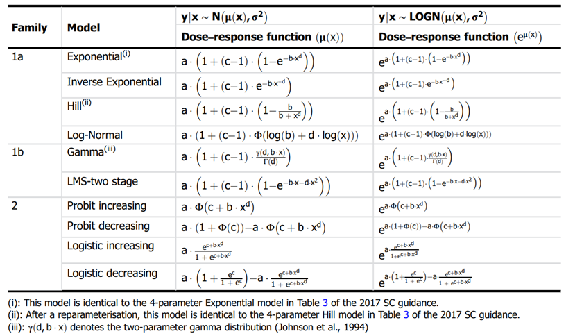
Candidate models for both distributional assumptions. The table has a header row with 4 cells. Each cell has split cells. Below there are 3 rows with multiple split cells. The table is shown in black and white.
Dose–response model for a single quantal endpoint
A quantal endpoint refers to a binary measurement: yes/no (typically coded as 1/0) according to the occurrence of a particular adverse event. As for a continuous endpoint, the statistical model for a quantal endpoint is defined by two components:
i) the specification of the distribution of the endpoint at a specified dose x. Only one distribution is possible (Bernoulli distribution).
ii) the description of the effect of dose on this distribution. Dose is affecting the probability on the adverse event.
Modelling the distribution
The main difference with a continuous outcome is that there is only one possible distribution for a quantal endpoint, the Bernoulli distribution; it has a single parameter, being the probability on the (adverse) event of interest. So, the first model component is uniquely defined as.
y|x ∼ Bernoulli(π(x)),
with π(x) being the probability on the adverse event at dose x. Note that π(x) is also the mean of the response.
Modelling the probability of an event
The dose acts on the probability π(x) of an event, typically considered as adverse. The same suite of candidate models as for the parameter μ(x) for a continuous endpoint is considered, with the restrictions that:
- They are only monotone increasing (as we expect the probability on the adverse event to increase with dose); contrary to continuous data, monotone decreasing data should be converted into increasing data, e.g. decreased survival could be transformed into increased mortality.
- The parameter representing the horizontal asymptote (c) is set such that this asymptote equals the value of 1 at infinite dose.
The three subfamilies of models for π(x) are:
- Family 1a and 1b: all models for μ(x) with c = 1/a, or
π(x) = a + (1 – a)F(x; b, d), b, d > 0,
for the same functions F as for Family 1a and 1b for continuous endpoints. The parameters a, b, d have a particular interpretation:
§ a = π(x) determines the background probability on the adverse event;
§ b and d characterise the shape of change in the probability on the adverse event, via the identity:
F(x; b, d) = πx-π(0) 1 -π(0) '
§ the model is reparametrised in terms of the parameter a (representing the background incidence), the BMD (the potency, see Table 3, and replacing the parameter b) and the parameter d.
- Family 2: all increasing models for μ(x) with c = 1, or
π(x) = F(a + bxd), b, d > 0,
for the same functions F as for Family 2 for continuous endpoints. The parameters b, c, d have a particular interpretation:
§ a = F-1(π(0)) determines the background probability on the adverse event;
§ b and d characterise the shape of change in the probability on the adverse event, via the identity:
bxd = F-1(π(x)) - F-1(π(0)),
§ the model is reparametrised in terms of the parameter c (representing the background incidence), the BMD (the potency, see Table 3, and replacing the parameter b) and the parameter d.
Table 3. Candidate models for quantal endpoints (Table from EFSA, 2017)
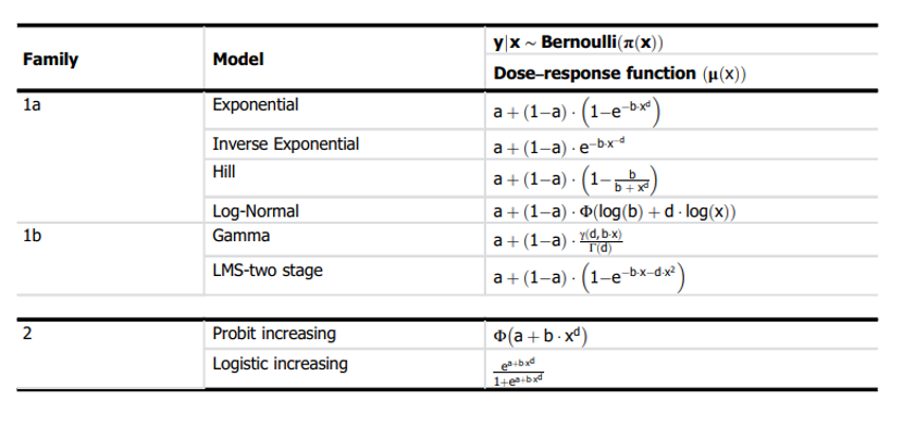
Candidate models for quantal endpoints. The table has a header row of 3 cells and 3 rows below. The rows all have split cells. The table is shown in black and white.
EPA 2022 - Benchmark Dose Software (BMDS) Version 3.3 User Guide
4. This section provides information about the statistical methodology and components of a dose–response model for a single continuous endpoint, and a single dichotomous endpoint as described in the EPA User Guide for the latest BMDS software (Version 3.3). The relevant information has been reproduced here verbatim:
Dose–response models for a continuous endpoint
Models in this section are for continuous endpoints, such as weight or enzyme activity measures, in simple experimental designs that do not involve nesting or other complications. The models predict the median value of the response, m(dose), expected for a given dose and the variation around that median. As evidenced by the previous discussion of the options available for continuous models, modeling of continuous endpoints requires consideration of more details than do those for dichotomous endpoints in similar designs. This section presents the mathematical and statistical details that determine how estimation is accomplished in BMDS.
The definitions of the continuous models are fully specified in the following table.
Note that 𝑚(dose) is the median response for the dose level specified.
Table 4. The individual continuous models and their respective parameters (reproduced from EPA User guide, 2022).
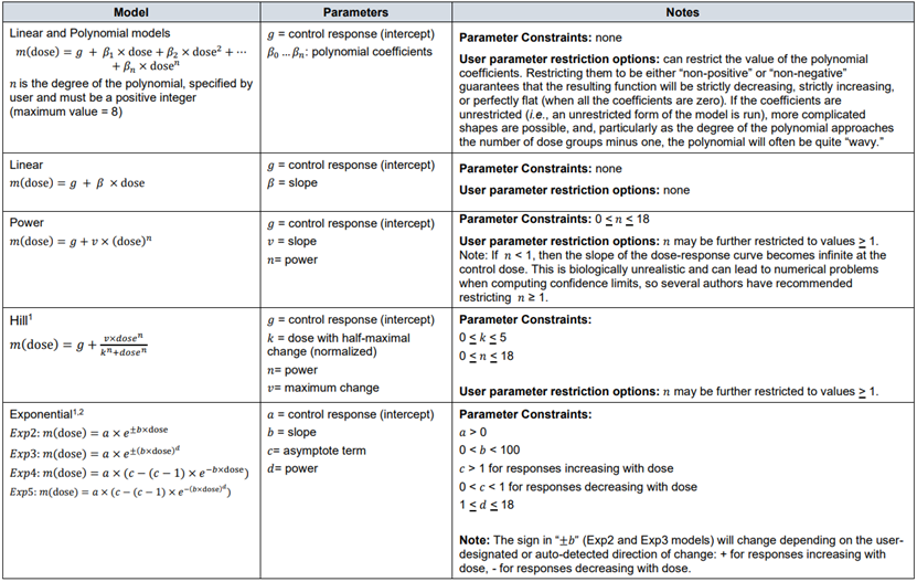
The individual continuous models and their respective parameters. This table is made up of a header row of 3 cells and 5 rows of 3 cells. The table is shown in black, white and grey.
1 BMDL estimates from models that have an asymptote parameter (including the Hill model) can be unstable when a wide range of parameter values can give nearly identical likelihoods. One indicator of that problem is that the estimated asymptotic response is far outside the range of the observed responses. The user should consult a statistician if this behaviour is seen or suspected. 2 RIVM (National Institute for Public Health and the Environment (Netherlands)). (RIVM, 2018). PROAST.
Note that the upper bounds for the power parameters in the Power, Hill, and Exponential models have been set to 18. That value was selected because it represents a very high degree of curvature that should accommodate almost every dataset, even ones with very (or absolutely) flat dose-response at low doses followed by a very steep dose-response at higher doses.
Dose–response model for a dichotomous endpoint
BMDS includes models for dichotomous endpoints in which the observations are independent of each other. In these models, the dose-response model defines the probability that an experimental unit (e.g., a rat or a mouse in a test of toxicity) will have an adverse response at a given dose. The actual number of animals that have an adverse response is assumed to be binomially distributed.
A specific example of such a dataset is a study in which adult animals are exposed to different concentrations of a toxicant and then evaluated for the presence of liver toxicity.
Table 5. The individual continuous models and their respective parameters (reproduced from EPA User guide, 2022).
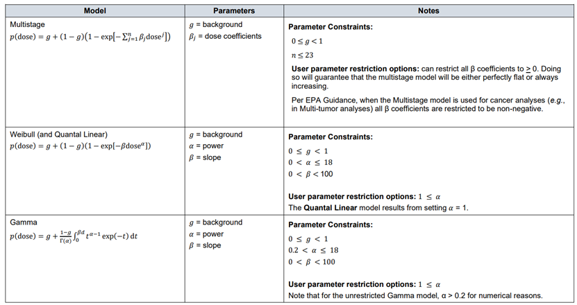
Dose–response model for a dichotomous endpoint. The image shows a table with a header row and 3 rows of 3 cells. The table is shown in grey, black and white.
Table 5 (continued).
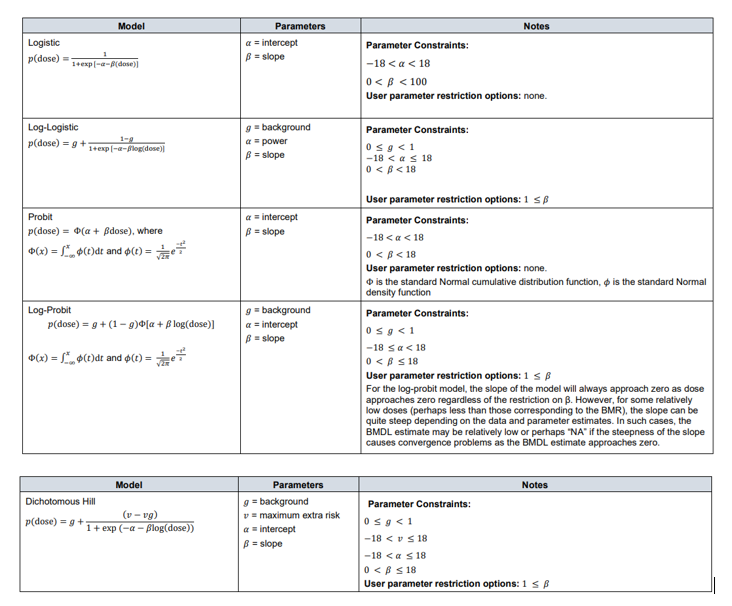
Dose–response model for a dichotomous endpoint. The image shows two tables both have a header row of 3 cells. The 1st table has 5 further rows, the 2nd table has only 1 row under the header row. Both are shown in black white and grey.
Note that the upper bound for the power parameter in some of the models, and the slope parameter for some of the other models, has been set to 18. That value was selected because it represents a very high degree of curvature that should accommodate almost every dataset, even ones with very (or absolutely) flat dose-response at low doses followed by a very steep dose-response at higher doses. If such parameter values are reported to be equal to 18 and/or the estimate in question is reported as “Bounded” (see the description of the output from dichotomous model runs in Section 11.5.2, “Analysis of Deviance Table,” on page 103), the parameter estimates are maximum likelihood estimates only in the restricted sense that the parameter in question has been assigned a value and the other parameters are MLEs conditional on that assigned value. Such model results are not strictly comparable with others in terms of AIC. In such a case, the BMD and BMDL could depend on the choice of power parameter; thus, sensitivity analysis is recommended if one intends to rely on the reported BMD or BMDL
References
EFSA, 2022. Guidance on the use of the benchmark dose approach in risk assessment. EFSA Journal 20, e07584. Available at: Guidance on the use of the benchmark dose approach in risk assessment | EFSA (europa.eu)
US EPA, 2022. Benchmark Dose Software User Guide Version 3.3. Available at: BMDS Version 3.3 User Guide (Oct 2022) | Benchmark Dose Software (BMDS) | US EPA